similarity learning
-
why similarity learning?
- we can’t solve all problems using regression or classification
- example - face recognition
- in general tasks like comparison, ranking and recognition need something more!
- if we used regression to predict a similarity score between 2 faces for example we would need to train our model for all possible pairs of faces which is impossible!
- if we used classification to recognize a person, we would need to train on every person which is not scalable!
- if we did a binary classification ex- {similar=0.2, different=0.8} we would need to run the model for all pairs of samples and the ranking would not be consistent meaning if A is similar to B and B is similar to C that does not mean A is similar to C!
-
how to define and quantify similarity?
- a positive function that returns a small value when x1 and x2 are similar and a large value when both are dissimilar
- we learn inverse similarity rather than similarity itself
- to determine matching pairs we use a threshold T
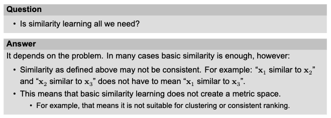
solution - constraint the distance D to be a metric - ie. produce a metric space
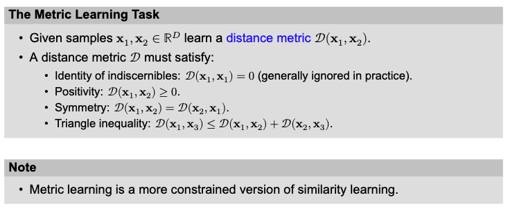

- Regression is not well suited because we cannot get direct labels
- Multi-class classification is not scalable and would not handle unseen classes at test time
- Binary-classification would not lead to consistent ranking as well as be inefficient
Mahalanobis Distance
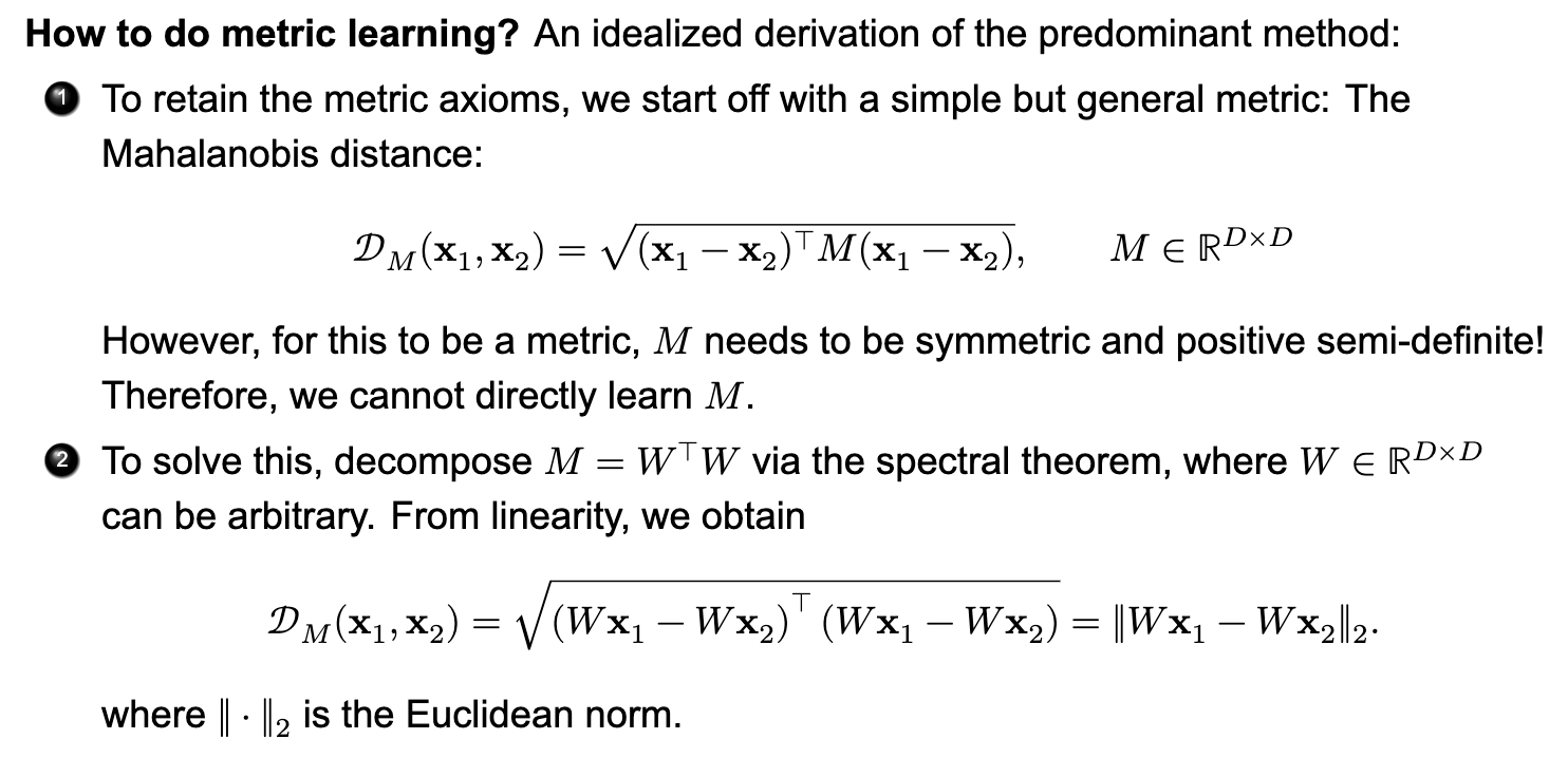
The mahalanobis dist warps, rotates, and scales our data space so that we can measure distances in a way that truly reflects the relationships between our data points.
M is the magic filter which is a square matrix that scales and rotates the space to account for the correlations and variances between different dim. M → +ve semi definite and symmetric
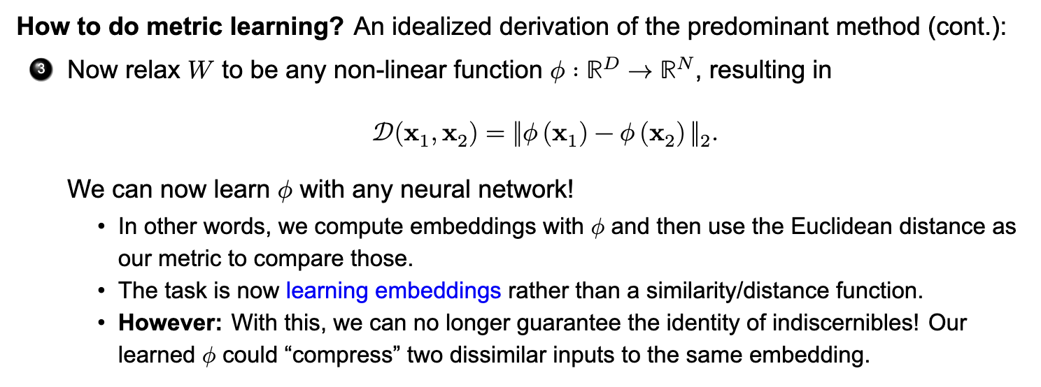
- Siamese Network
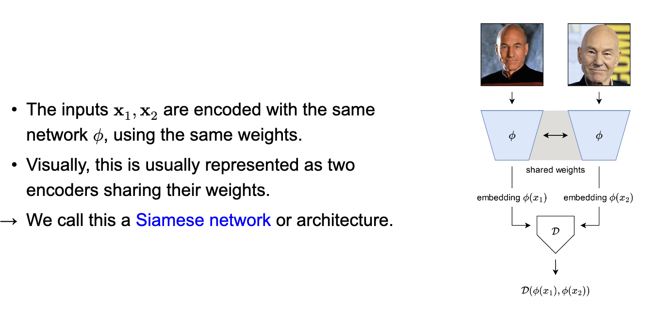
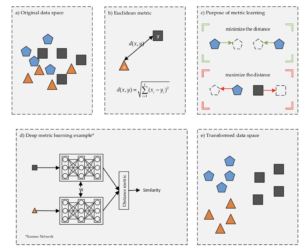
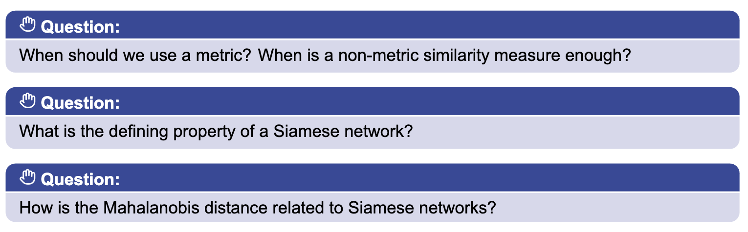
- We must use a metric space or triangle inequality eg. consistent ranking, clustering etc
- Siamese n/w - we process both inputs with the same encoder which have the same shared weights
- We can decompose the matrix M into M=W^T T and then generalize W to any non-linear encoder phi
contrastive learning
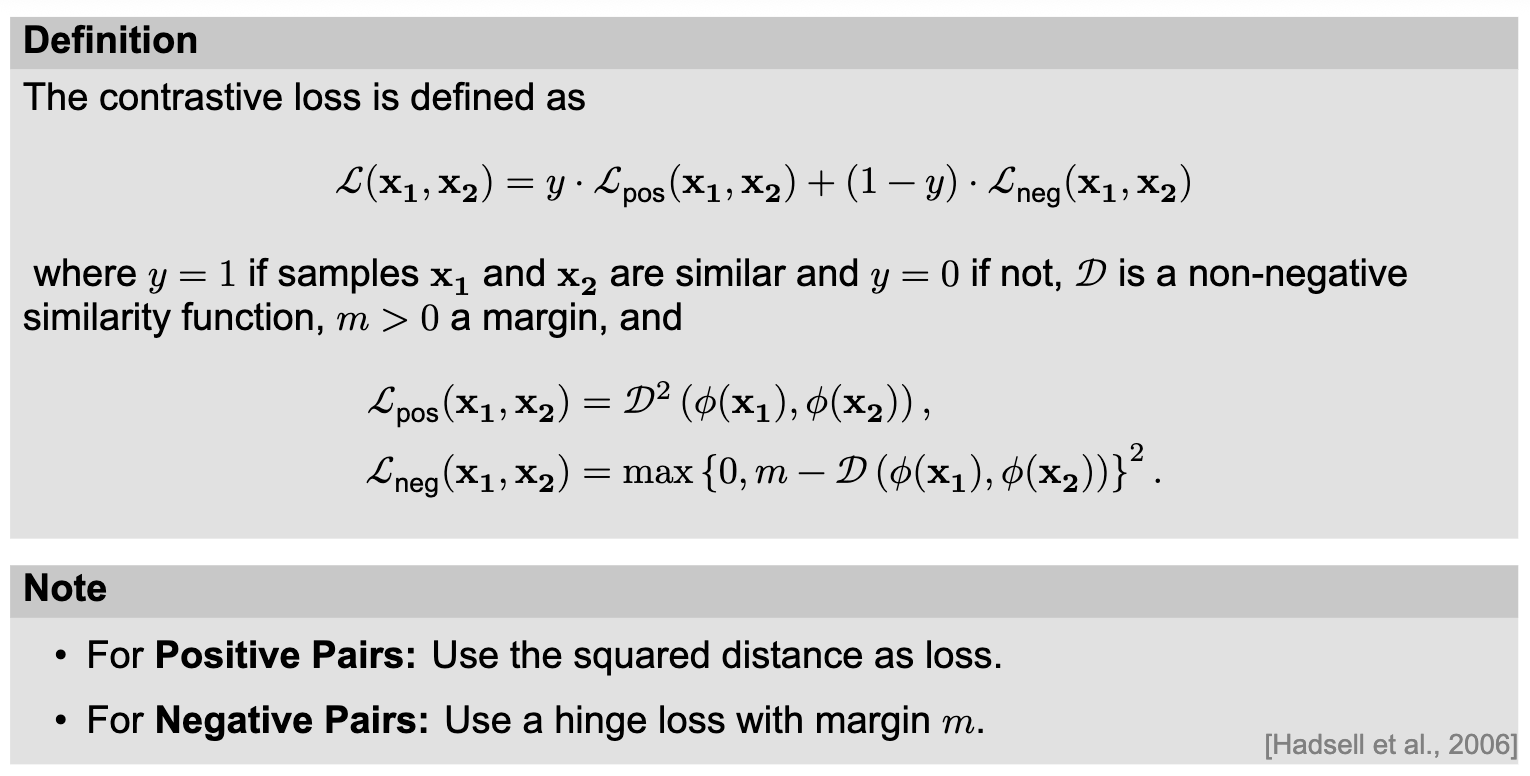
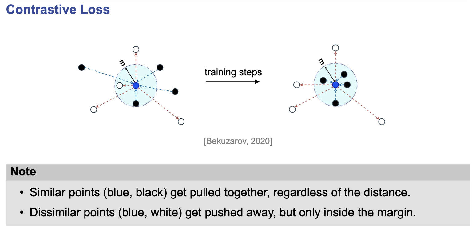
Note:
- We can compute gradients and weight updates independently for each encoder
- we just need to average them afterwards
- contrastive losses are essential for:
- representation learning
- self-supervised learning
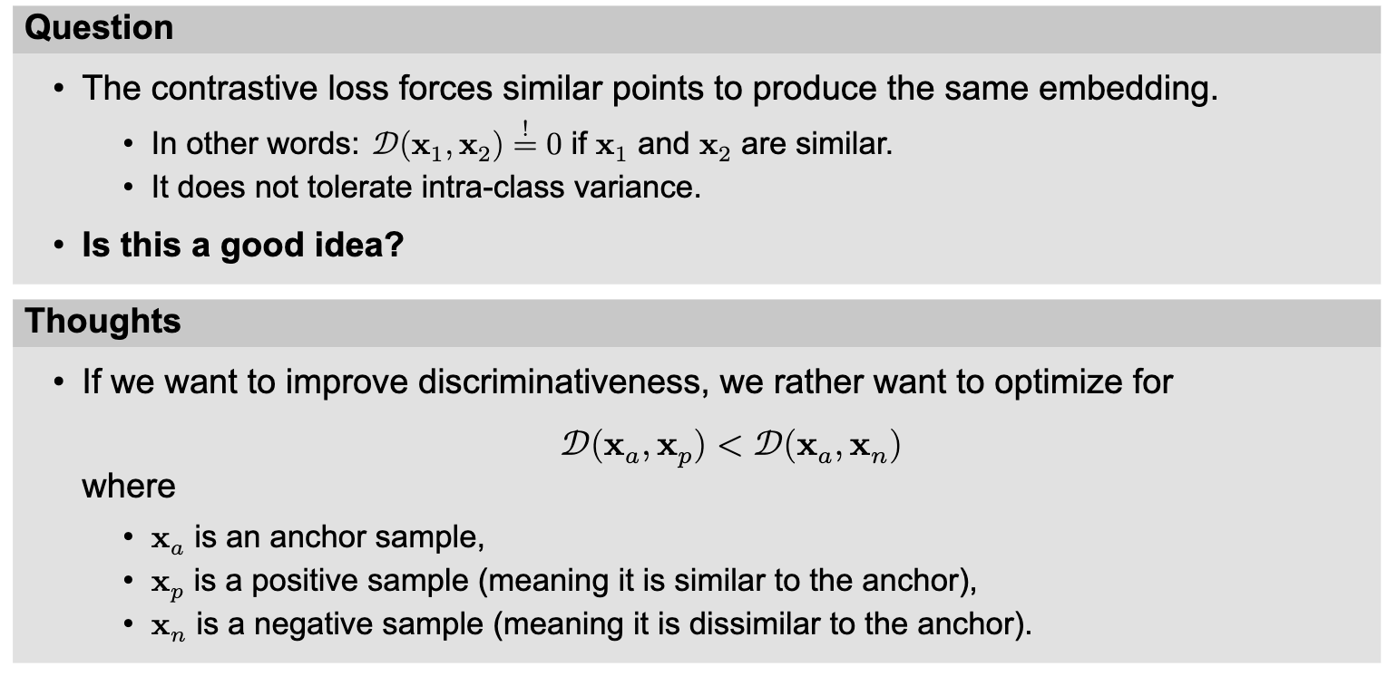
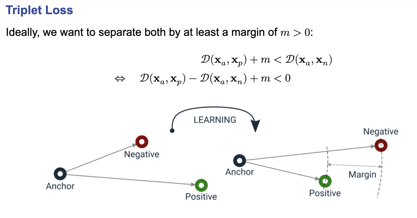
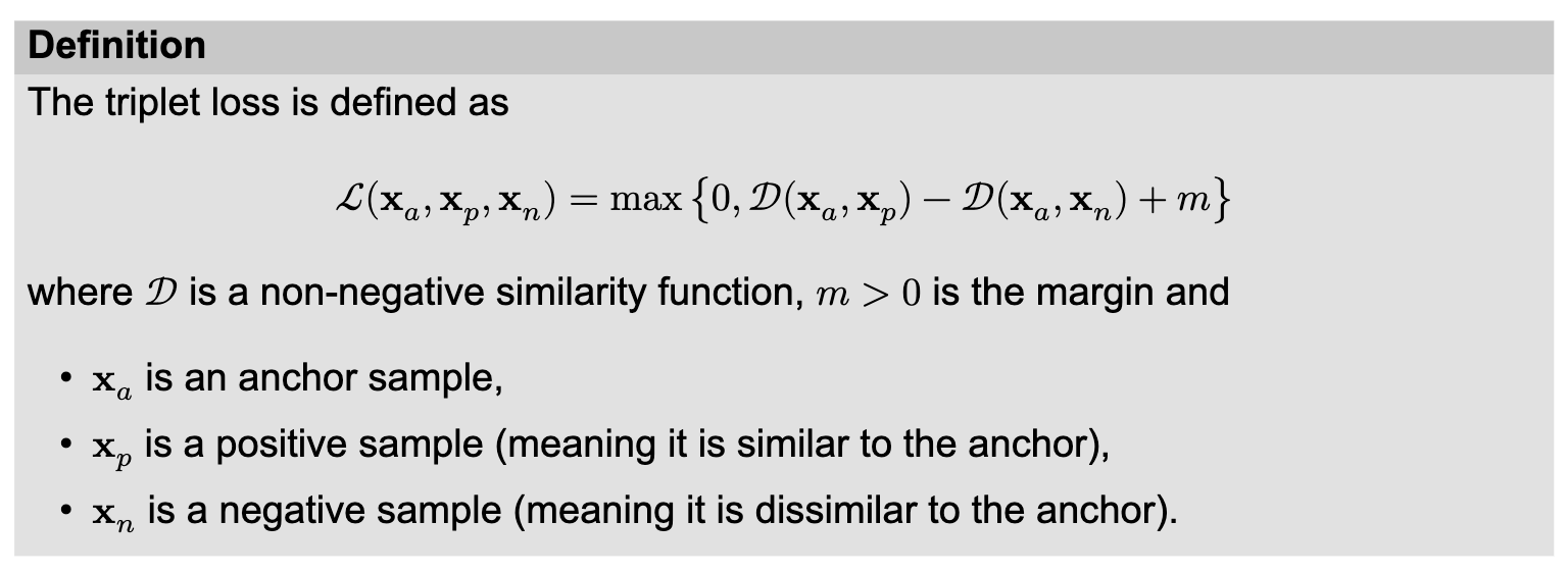
- Triplet loss is more powerful than the contrastive loss
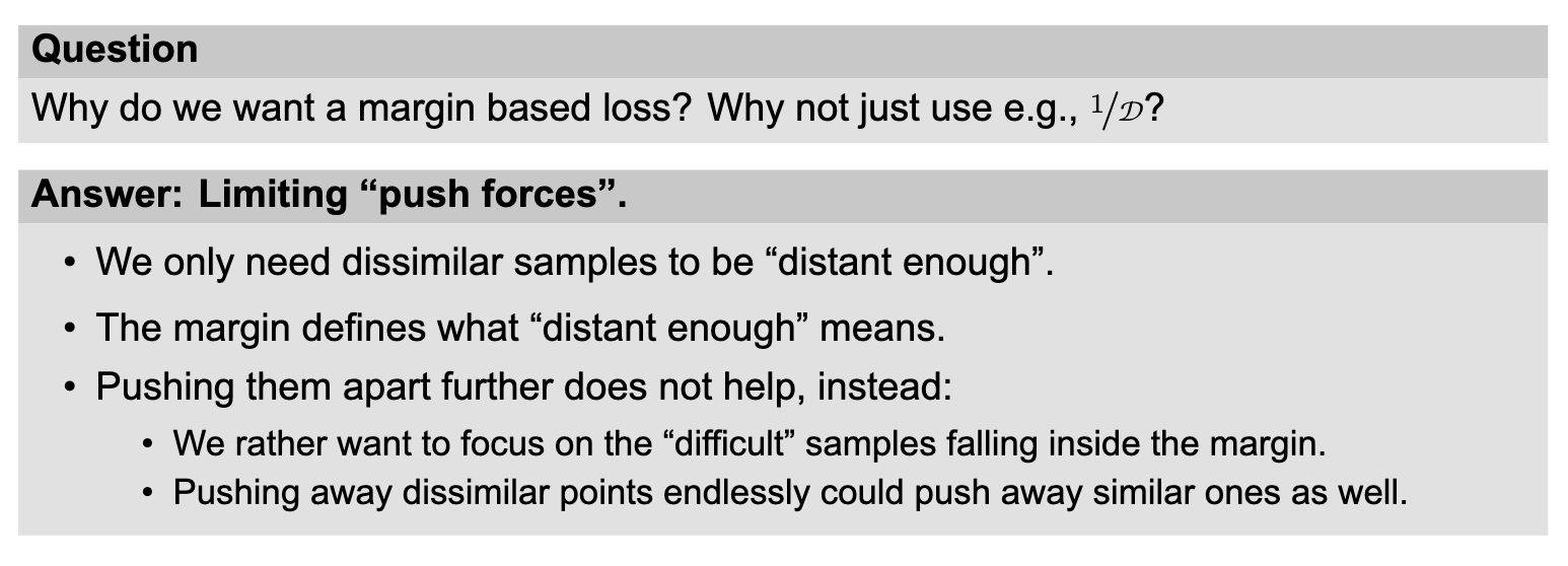
- it allows for more intra-class variance and doesn’t force embeddings to be equal but only requires that there is a margin m between different samples
- We need to sample both +ve and -ve pair so negative mining is essential to make it work!
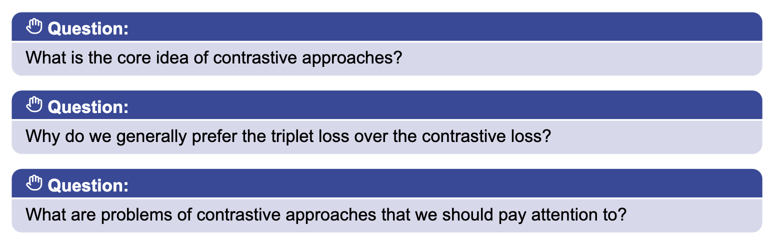
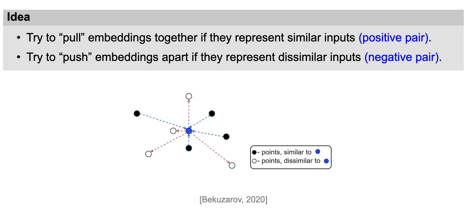
- pull together similar samples in the embedding space, push away different ones!
- the triplet loss allows for intra-class variance and only requires that there is a margin between +ve and -ve samples. The contrastive loss does not and basically tries to pull similar samples into the exact same location, this can lead to sub-optimal results
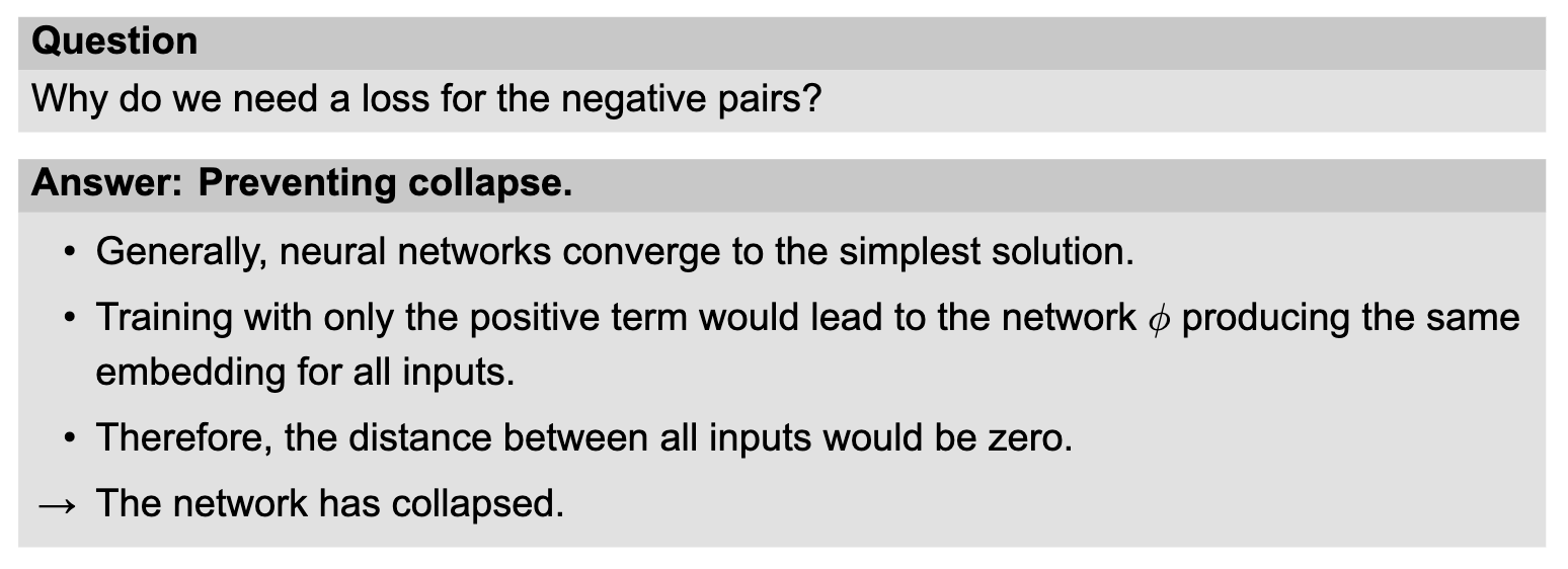
- network collapse, sampling
sampling and sample mining
-
for triplet loss with a dataset of size N, we have O(N^3) possible triplets → training with all is computationally infeasible
-
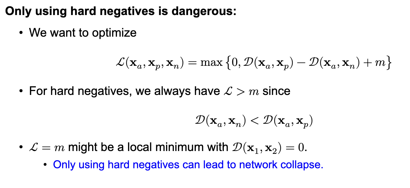
we require triplets that fulfill D(xa, xn) < D(xa, xp) + m otherwise Loss_triplet=0 and the model will not learn anything
-
negative samples can be classified as:
- easy negatives - where the loss=0
- semi-hard negatives - where the -ve points are within the margin
- hard-negatives - where the -ve points are misclassified
- common practice - use both hard and semi-hard negatives
-
why we cannot use only hard negatives?
-
The most valuable samples are semi-hard negatives ie 0 < Loss < m
-
Offline Mining - generate a list of possible triplets offline and sample from that
- make a checkpoint of the model
- use that to compute embeddings for a subset of the dataset
- generate new triplets using the computed embedding
- train with these triplets for the next N steps (or epochs)
- repeat from step1
-
Offline Mining - problems
- we need to compute M= N.3 embeddings in worst case for N triplets
- need to compare each +ve pair to all other embeddings O(M^3)
- doing this on whole dataset is infeasible
- we need to re-compute the embeddings again during training
-
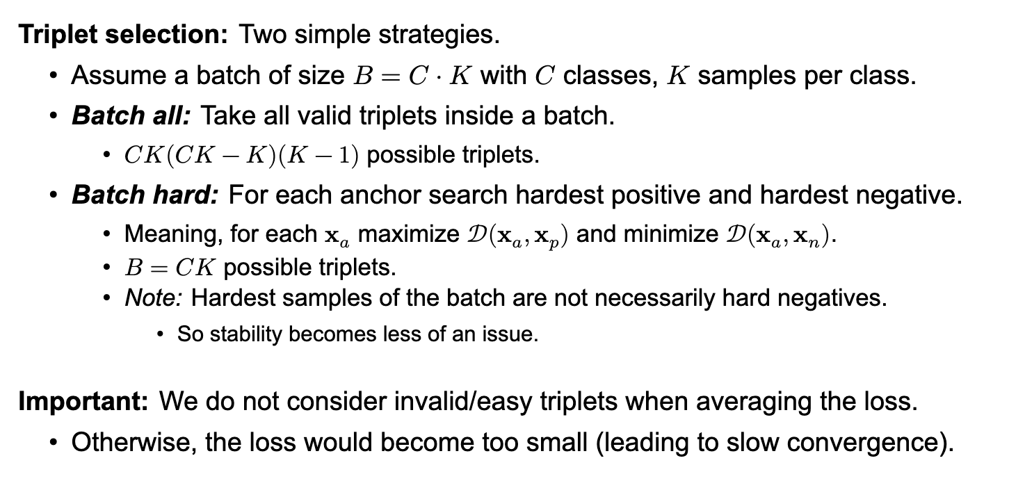
Online Mining - Mine triplets on the fly from each batch while training
- take a batch of size B
- look at all the possible triplets in that batch (less than B^3)
- select a subset of valid ones
- compute loss and perform back-propagation only using those
-
each batch should contain a min number of samples of each class otherwise positive pairs will not be well-represented
-
we can construct a batch by sampling K samples for each of the C classes
-
it is important because it has direct impact on the quality of solution and the convergence speed. With some triplets we cannot train at all and with others the network might collapse
-
it can lead to network collapse, as the network might shortcut learn to just output the same embedding for all points
-
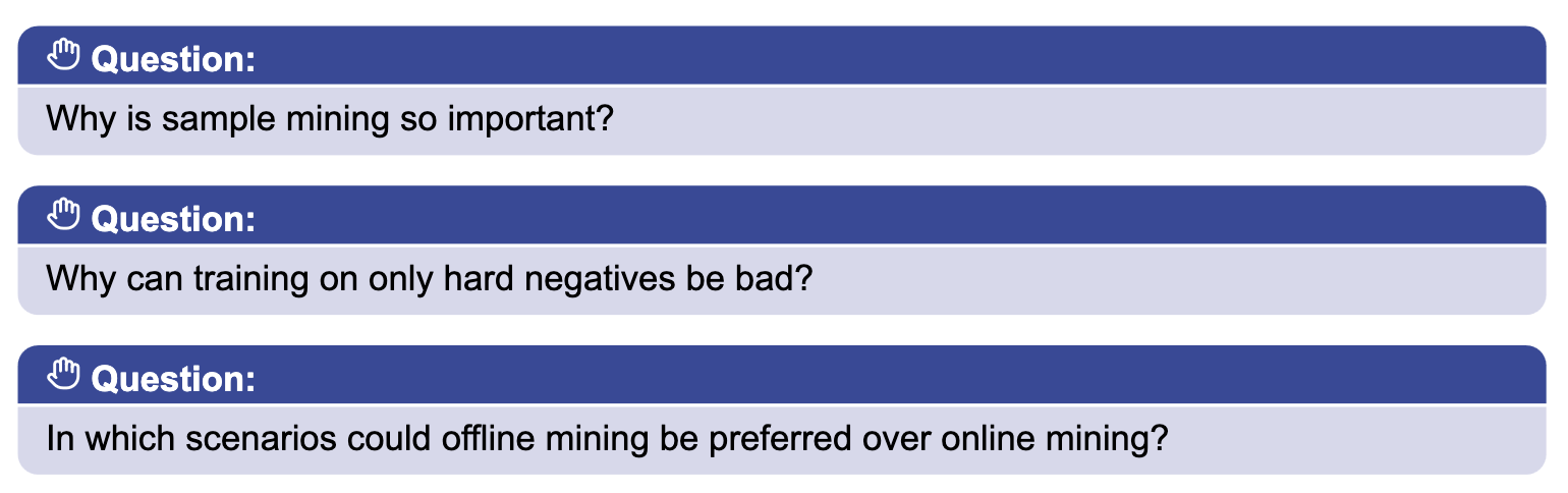
when we are constrained in batch size or have huge number of classes that we cannot adequately sample and pack into a batch, such that +ve and -ve are well reflected
beyond contrastive methods
-
There are 2 major problems in contrastive learning
- expansion problem:
- majority losses only act locally (eg the triplet loss is limited to 3 samples)
- severely limits the global impact of the loss.
- no guarantee that all similar samples end up close to each other.
- sampling problem:
- contrastive approaches rely strongly on sampling (convergence, optima)
- we want to find the most useful samples - as some do not contribute at all
- expansion problem:
-
Classification
- we use the learned embeddings and add a linear layer and softmax to our encoder and use the categorical cross-entropy loss for training
- softmax loss
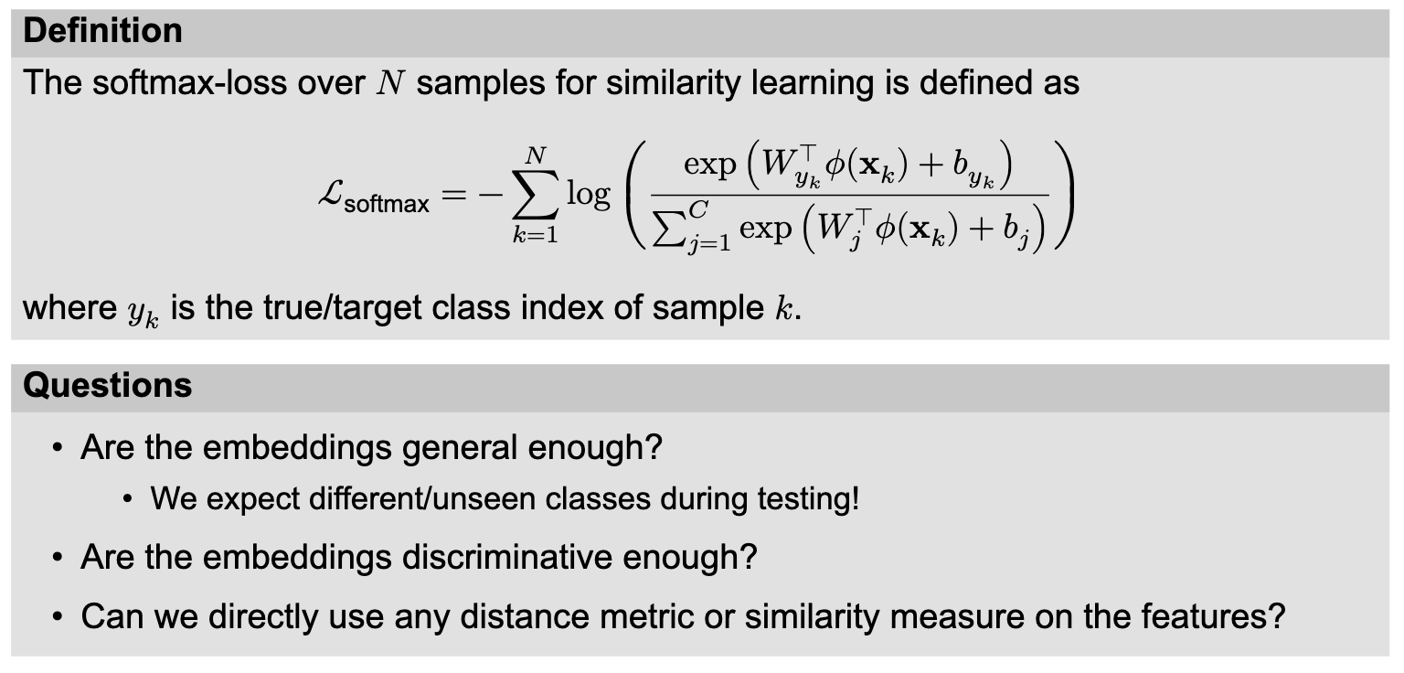
- training using this method in a toy example like the MNIST shows us that although the classes are separable there is significant intra-class variance which means the embeddings are not discriminative enough hence this method is not very well suited for distance functions
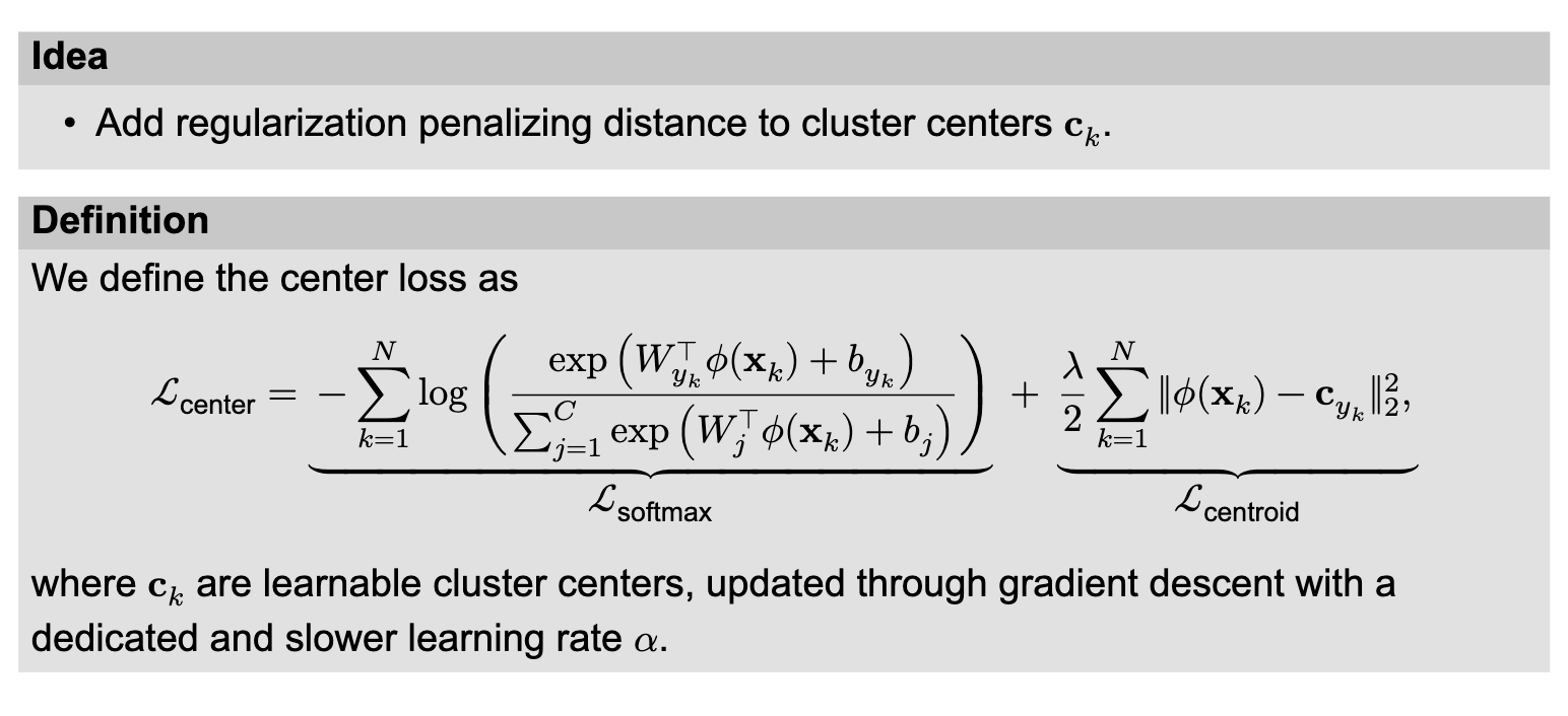
- we can use Center loss:
 Note:
- training only with a softmax loss would lead to large intra-class variance
- training only with centroid loss would lead to network collapse
- we need both
- Original paper suggests incorporating a PCA:
- perform PCA on the training embeddings
- transform embedding during test time using that
- compute cosine similarity on embeddings after the PCA
- could help with unconformity between both loss terms
Center loss: - solves the expansion issue - class centers pull clusters together - avoids the sample mining problem: - we just train with individual samples - there is no need to mine pairs or triplets - Inter class distance can still be small - only intra-class distance is penalized
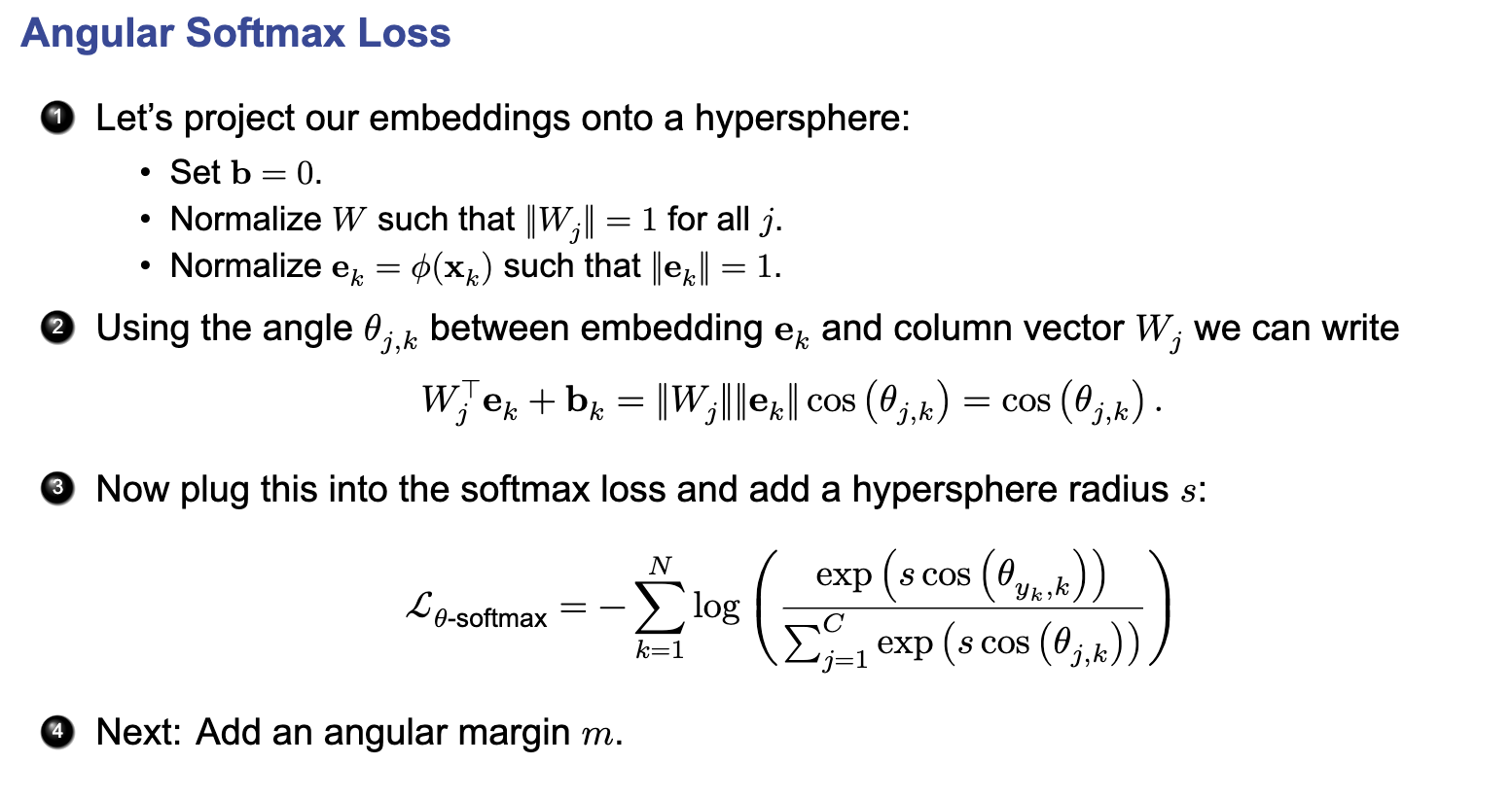
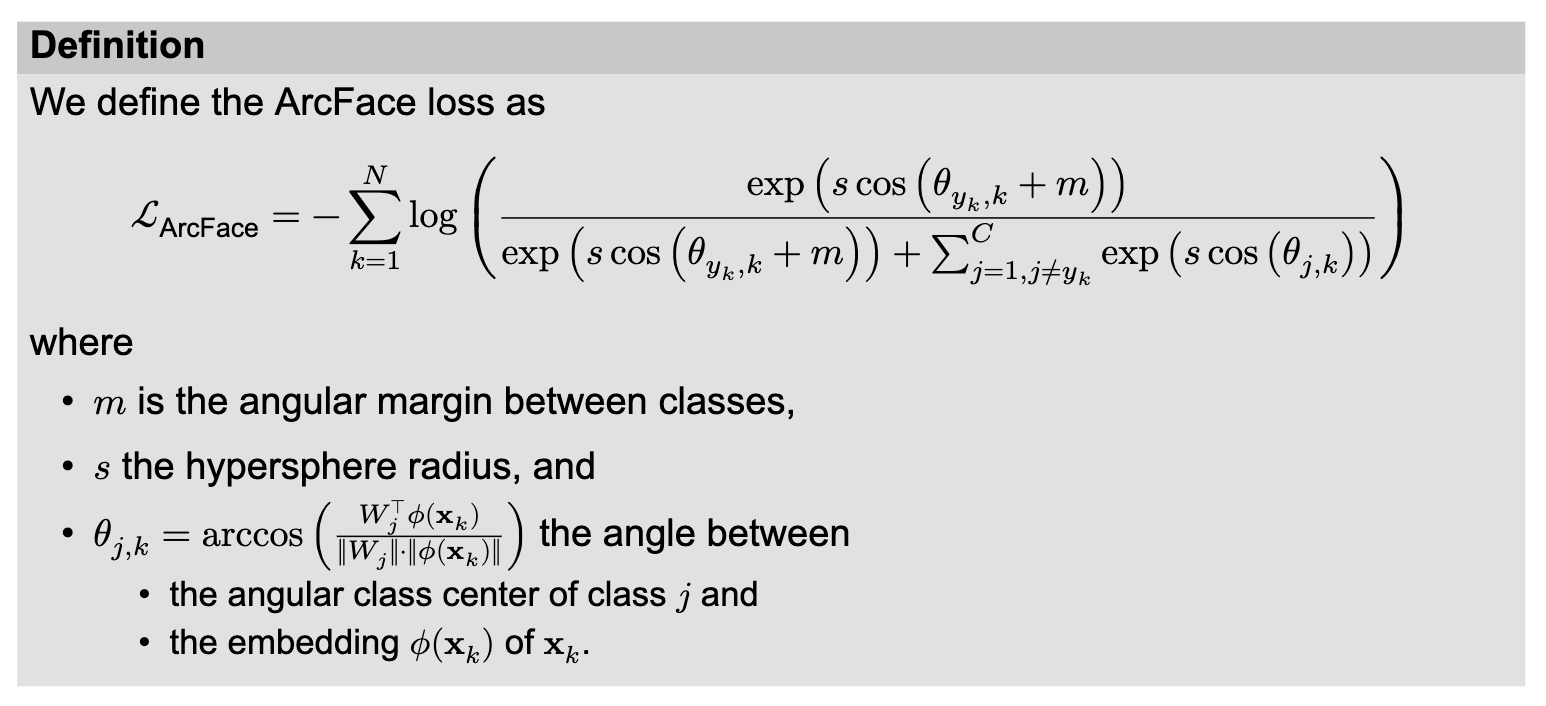
- calculate similarity directly via the cosine similarity between embeddings
- solves expansion issue
- bypasses sampling problem
- retains inter-class distance via angular margin
Contrastive vs Angular Margin Methods:
- Angular margin methods more powerful as they bypass the sampling problem
- they largely solve the expansion problem
- both are inherent with contrastive methods
- however we need to know class labels (cannot be used in unsupervised or self-supervised)
- do not react well in OOD
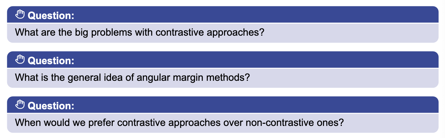
- expansion and sampling
- project the embeddings into a hypersphere and enforce an angular margin clusters of classes
- when we do not have labels, for OOD data
Links:
202609070039