generative models
- generates o/p but many o/p valid
- if we know p(x) we can sample x ~ p and also estimate the likelihood of o/p
- p(x) does not have to be known explicitly!
- conditional generation - p(x|c)
- diff b/w generative and discriminative models
- discriminative - p(y|x) → only 1 true label y for each input x (many-to-one) ex- classification
- conditional generative - p(x|c) → many valid outputs x for a condition c - (one-to-many or many-to-many)
- formulating generative modeling
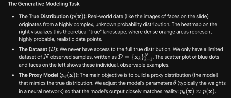
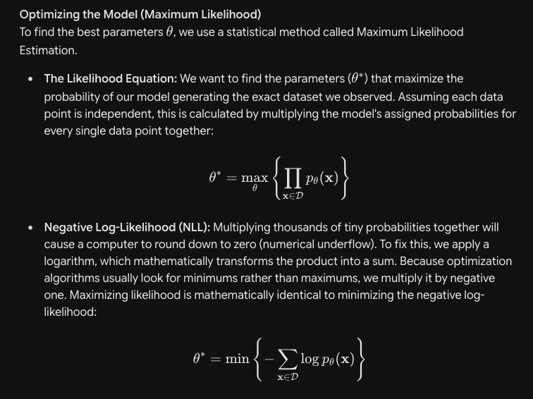 Maximizing likelihood = Minimizing -ve log likelihood
-
implicit vs explicit representations
- explicit - directly learn the probability density function using max likelihood estimation method ex- VAEs, Autoregressive GPT etc.
- implicit - bypass the need to calc exact probability numbers, the dist is learned within the model’s weights, instead focus on generation ex- GANs
-
Types of Generative Models:
- Autoregressive Models
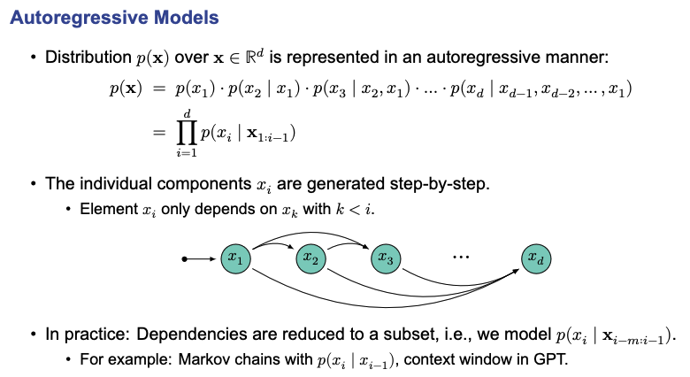
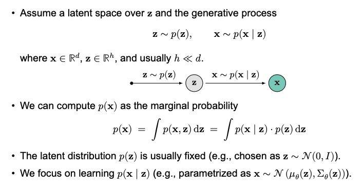
- Latent Variable Models
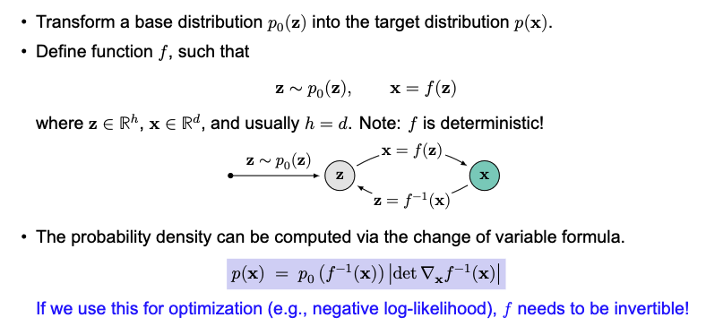
- Flow-based Models
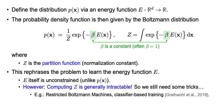
- Energy-based Models
- Autoregressive Models
-
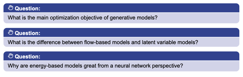
main objectives of generative model is to minimize -ve log likelihood
-
flow-based models - does not need a latent space, takes an intial dist → o/p dist.
-
latent variable models - sample a latent variable z and then conditionally generates the output based on the prior z.
-
directly allows to learn the energy function via NN, the exponential function ensures positivity and partition function ensures normalization.
-
Problem with partition function? → computing it is intractable!
-
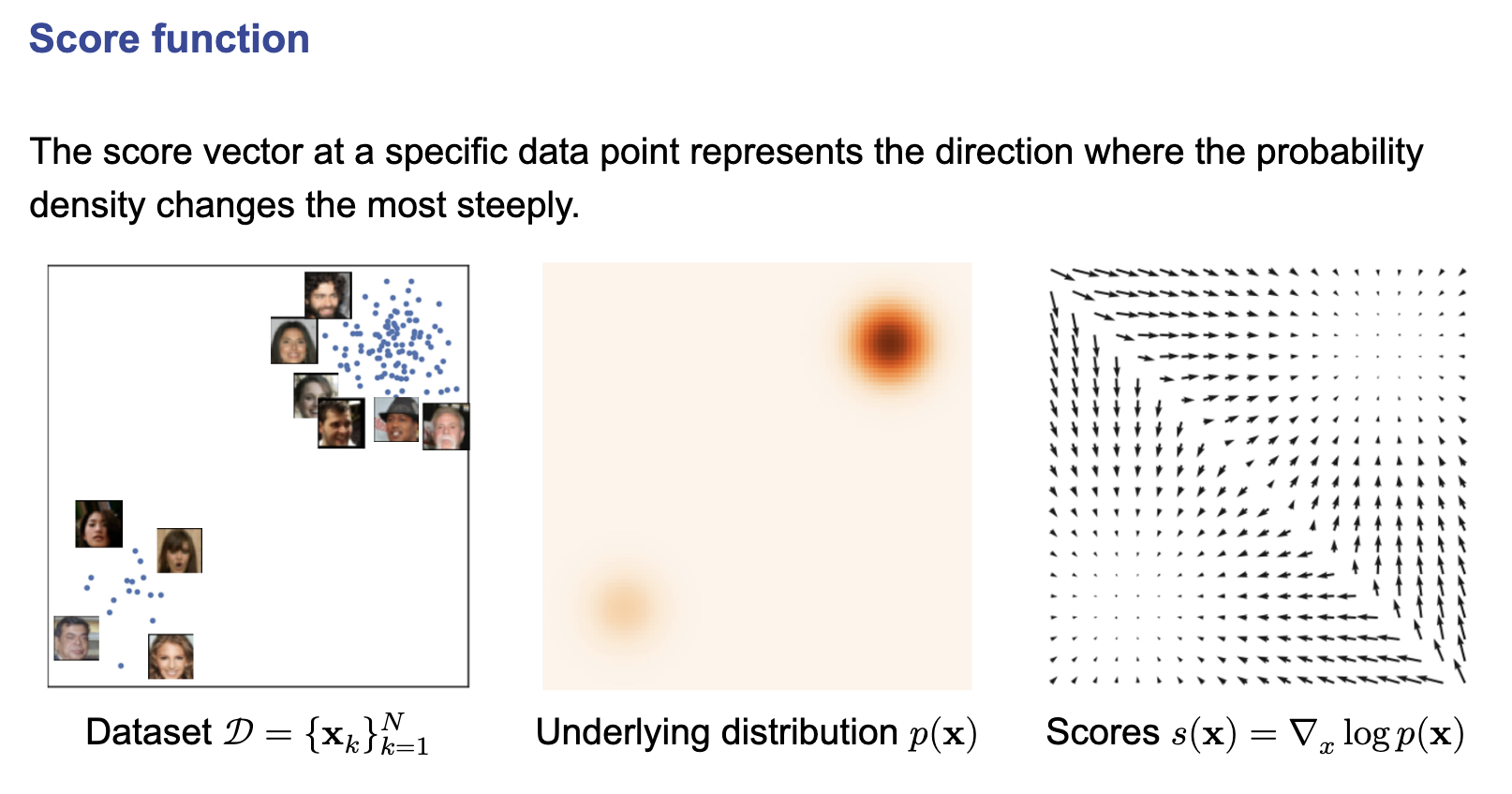
how to avoid the partition function? gradient of the log p(x) is the score function of p wrt to x
-
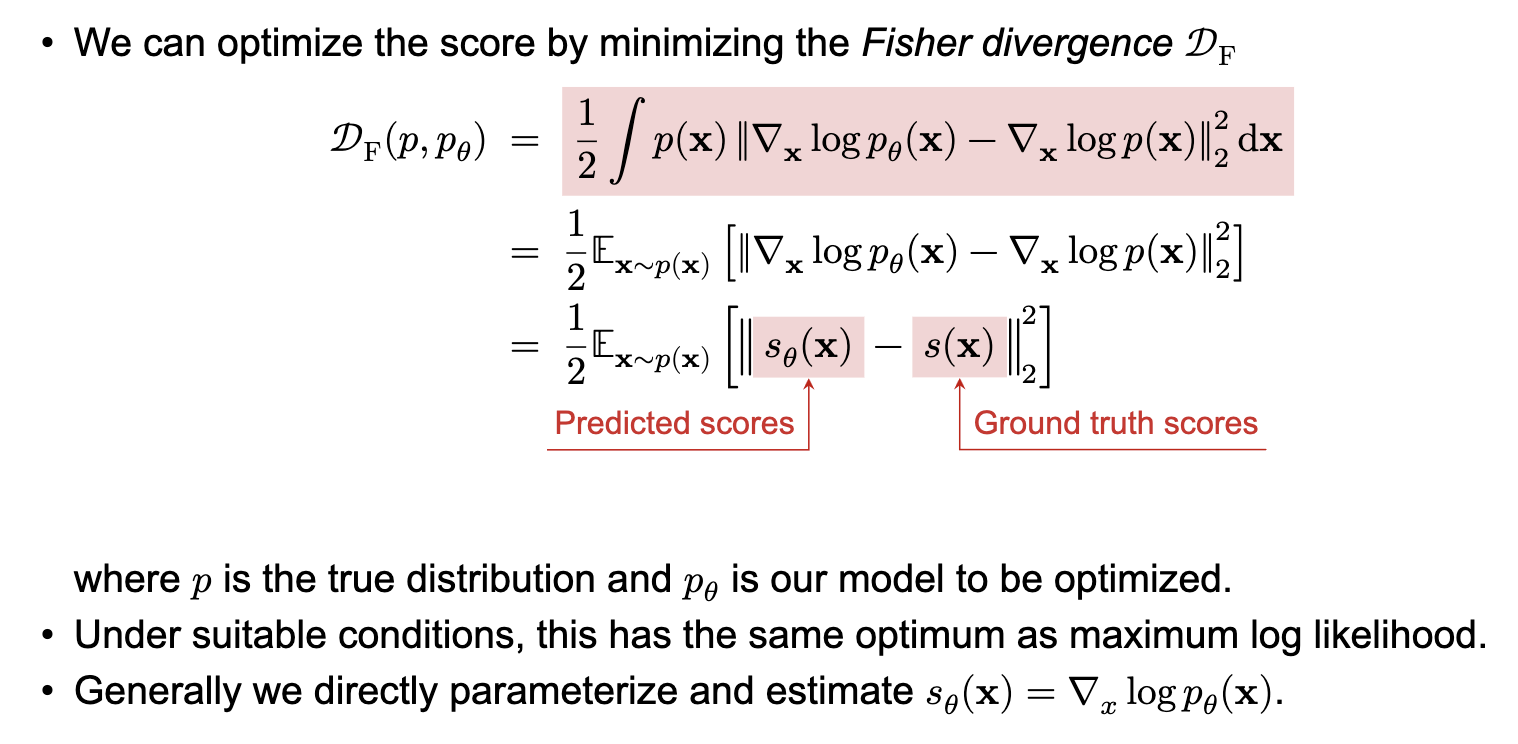
we can optimize the score (which is independent of the partition function) by minimizing the Fisher divergence which has the same optimum as the max log likelihood
-
Denoising Score matching
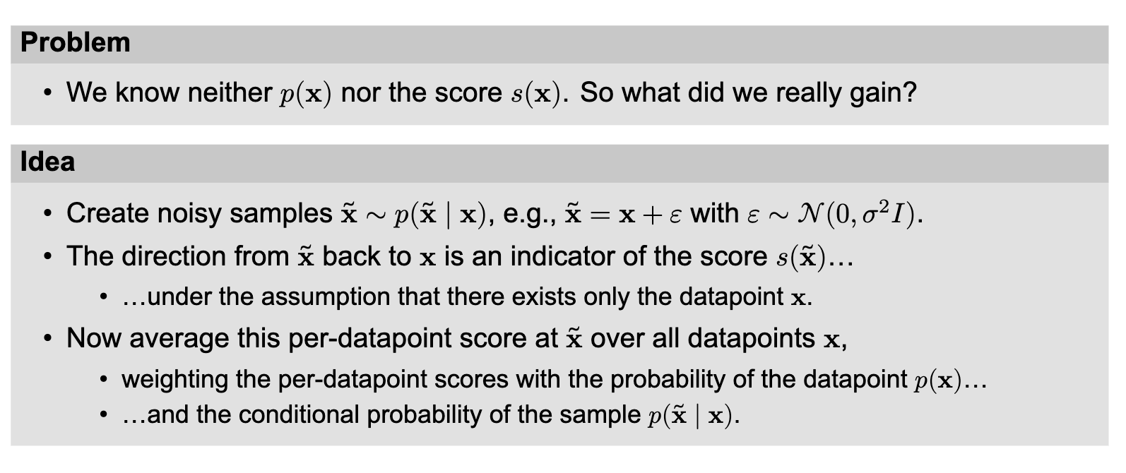
- in order to bypass Z, we take the gradient of the log-likelihood w.r.t input x, this derivative is called score function. The score vector at any specific data point points in the direction where the probability density increases most steeply!
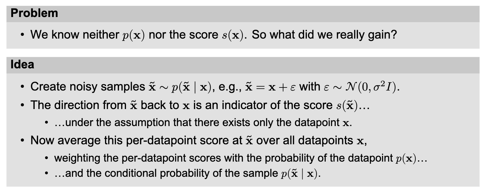
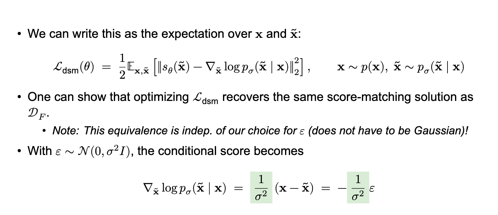
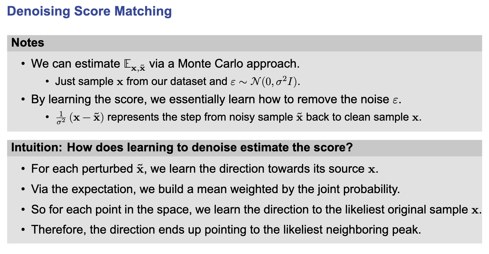
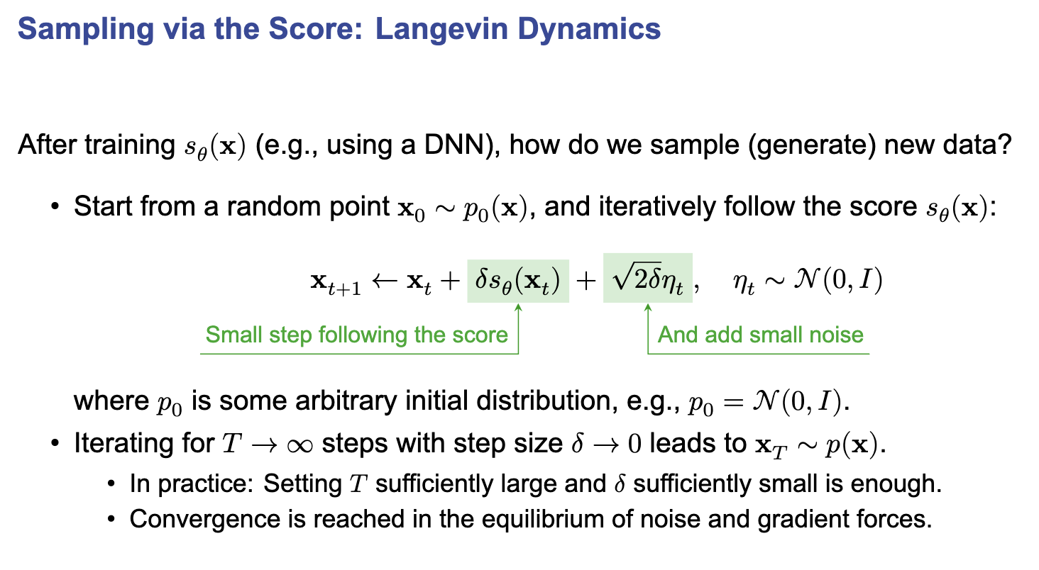
- we must add a small noise to avoid the convergence case!
-
Noise Conditional Score Networks (NCSN)
- for regions with low-density, the noise based score estimate is inaccurate so we artificially enlarge the dist by adding stronger noise
- large noise corrupts data, so we use multiple noise levels, in training we sum up the losses over noise levels
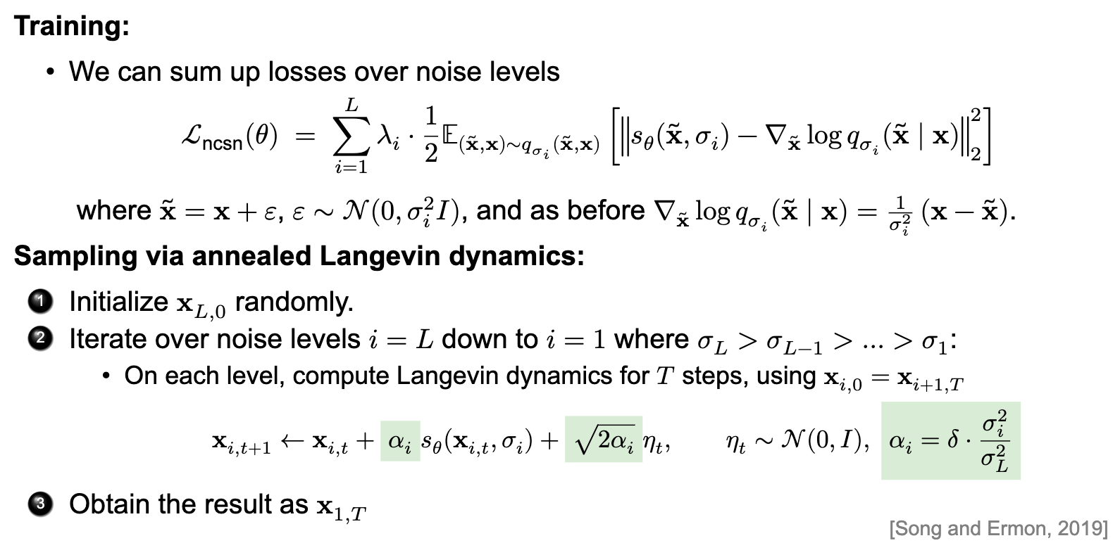
-
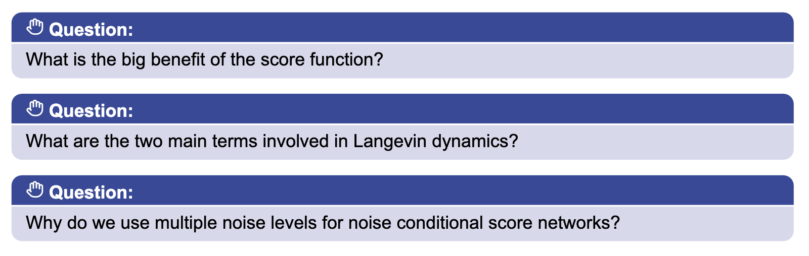
benefit → we do not need to deal with the partition function as the score does not depend on normalization constant and since the score is real values function without any constraints, it can be directly approximated by a neural network
-
score (moves the sample towards more probable region of the target dist) and the noise level (required to actually model the dist)
-
because for lower noise, the density is lower at many regions causing inaccurate score estimates, but since larger noise reduce acc, use both large and small noise!
-
Diffusion models
-
Denoising Diffusion probabilistic Models
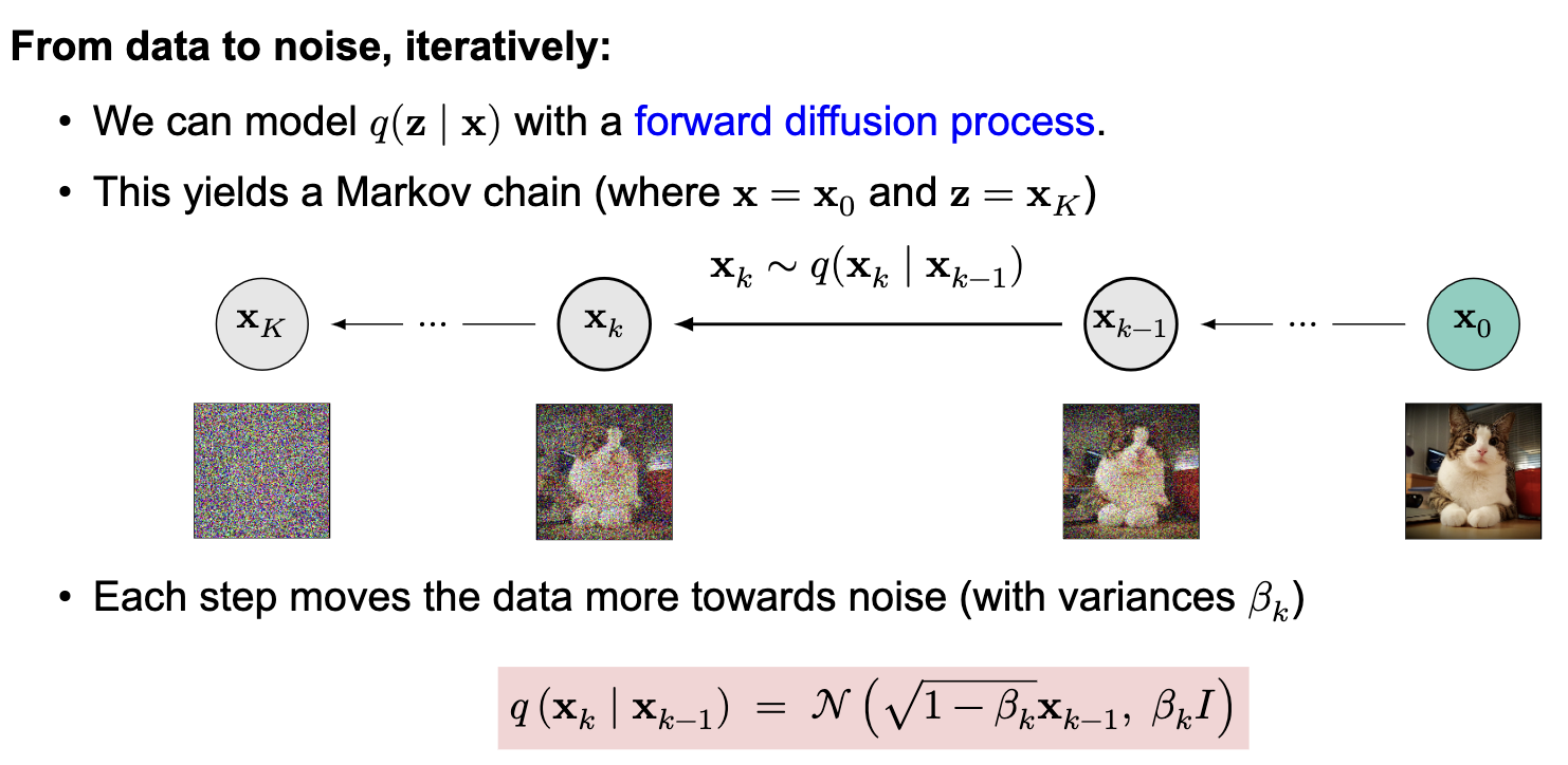
- we first try to learn how to create noise from data q(z|x)
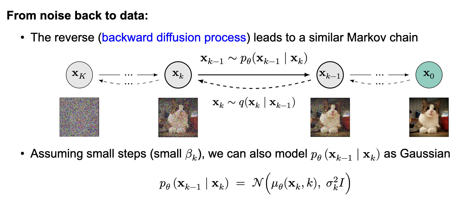
- then we try to reverse learn how to obtain data p(x|z) from q(z|x)
- similar to variational auto-encoders but trying to learn in a single step is difficult hence we break it into smaller, iterative steps that are easier to learn
- q(z|x) is called forward diffusion process which yields a markov chain
- from noise to data - backward diffusion process leads to a similar Markov chain
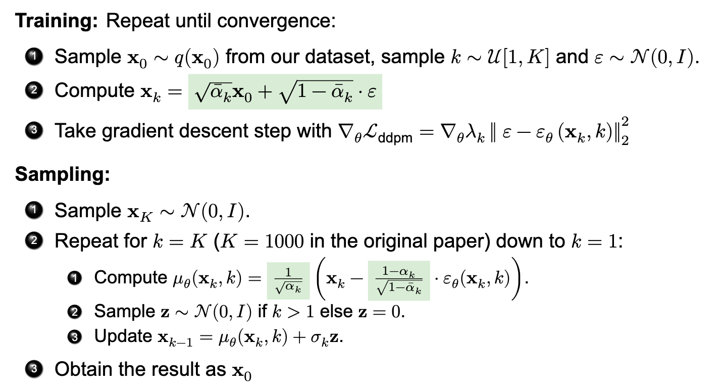
- Training a DDPM → predicting the noise contained in a noisy sample!
- DDPM is score matching!
- training with denoising objective
- the update step is however different from the denoising score matching problem
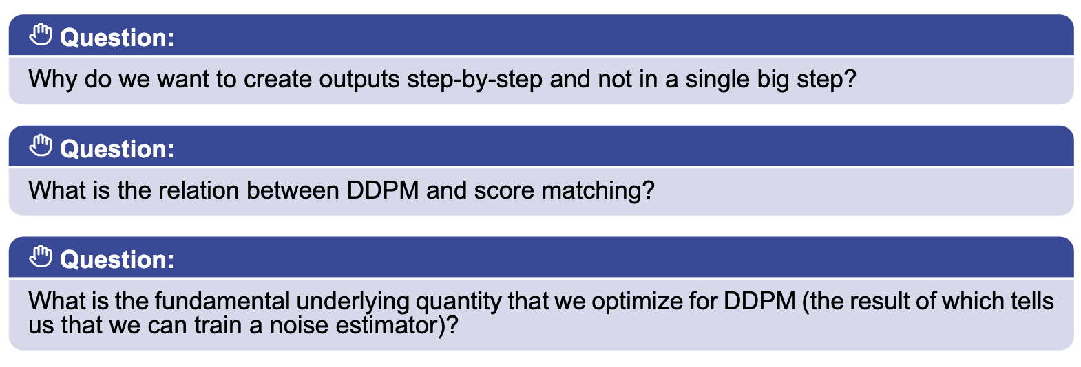
- because it is easier for the network to learn small denoising steps. From pure noise, it is hard to infer a realistic sample in one shot, taking small steps is much easier!
- both add noise to the original sample and try to denoise it, in DDPM the model predicts the noise that was added to x, this predicted noise is directly related to the score of the noisy distribution, which connects DDPMs to denoising score matching and score-based models
- approximated with a lower bound, it tells us that we can optimize it by training a noise estimator
-
Continuous-time Diffusion
- infinitely many steps, taking dt=0 leads to SDE - Stochastic Differential Equation
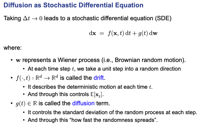
- Reverse process - we start with random noise at t=1 and solve the SDE backwards in time to t=0
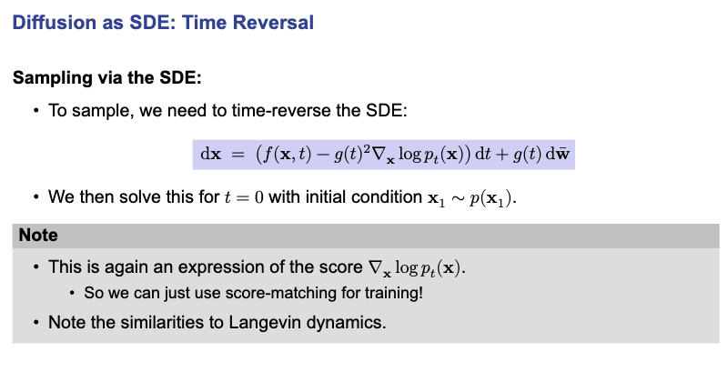
- Our SDE has a corresponding ordinary differential equation (ODE) inducing the same Pt(x) called probability flow ODE which is deterministic and no stochastic process is needed.
- Discretizing the ODE leads to Denoising Diffusion Implicit Models
- Benefits of ODE:
- no random noise is injected during generation which allows for completely deterministic sampling paths!
- discretizing the ODE yields Denoising Diffusion Implicit Models (DDIM)
- bridges diffusion models to CNF and flow matching
- infinitely many steps, taking dt=0 leads to SDE - Stochastic Differential Equation
-
Diffusion - conclusion
- diffusion is basically training a denoiser or noise eliminator
- usually implemented as a single network with time as input (S(x,t)) where t is encoded using sinosudal embeddings (or similar)
- sampling and training are disjoint (so we need to scale and reparameterize accordingly)
-
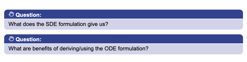
SDE formulation allows us to choose f and g flexibly
-
we can use any ODE solver and since it is deterministic, it allows interpolation in the latent space!
-
Guidance methods
- until now we saw models that generated a random sample from a dist but in reality we want to generate something using a text prompt or a condition!
- classifier based guidance methods use bayes rule to get score
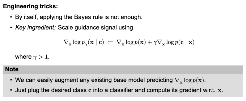
- problems:
- the classifier deals with noisy inputs (so we need to train the classifier)
- guidance can be only applied to known classes!
- classifier free guidance
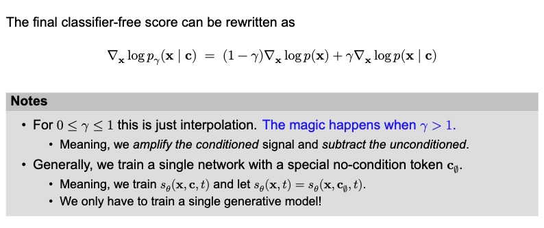
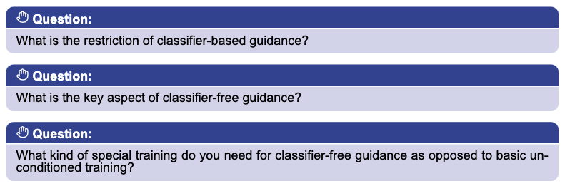
- we need to compute dx(log(c|x)) which requires classifier trained on noisy inputs, this limits us to known conditioning formats or fixed set of classes.
- we amplify the conditioned signal and subtract or remove the unconditioned signal
- we need to train a conditioned score estimator, which does not depend on the condition scale gamma!
-
-
Diffusion in Practice
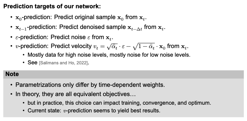
- Loss formulation
- likelihood based derivation gives time-step weights alpha for loss terms
- noise schedule
- the choice of noise can significantly influence output quality
- samplers
- stochastic vs deterministic
- SDE and ODE
- diffusion specific solvers take advantage of ODE structure!
- Loss formulation
-
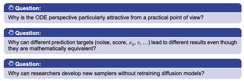
Diffusion process is an ODE hence it is easy to use existing ODE solvers which gives access to many numerical methods and allows us to trade off sampling speed against accuracy!
-
they are equivalent only upto transformations, during optimization, however different parametrization lead to different loss landscapes, gradient magnitudes and convergence behavior
-
training and sampling are decoupled, as long as the sampler can work with learned representation, for example a noise or score estimate, different sampling strategies can be applied to the same trained model.
-
Continuous Normalizing Flows and Flow Matching
- we defined normalizing flows as invertible transform f with x = f(z) where z ~ p0(z)
- since learning a single function f is complicated we split it such that each step is invertible
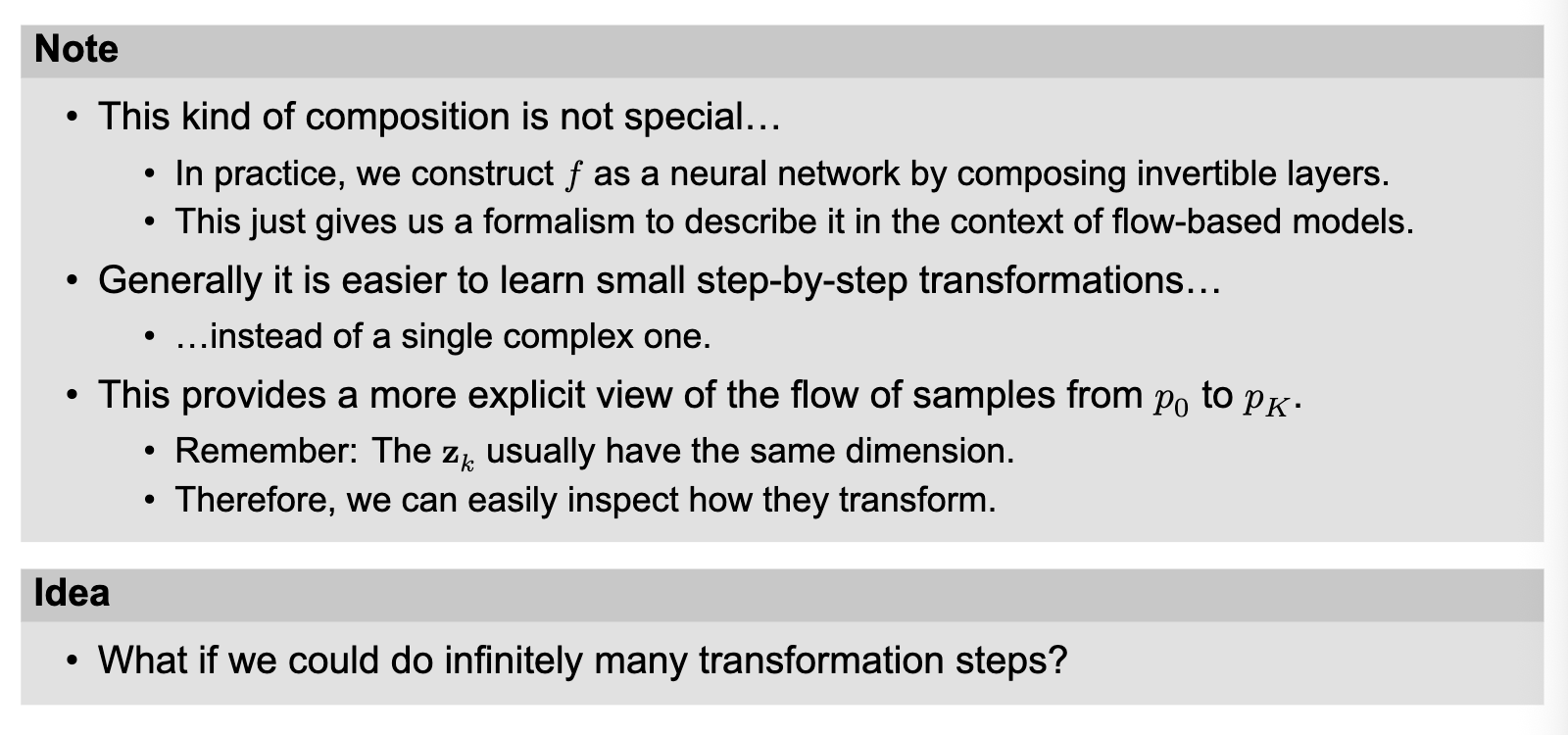
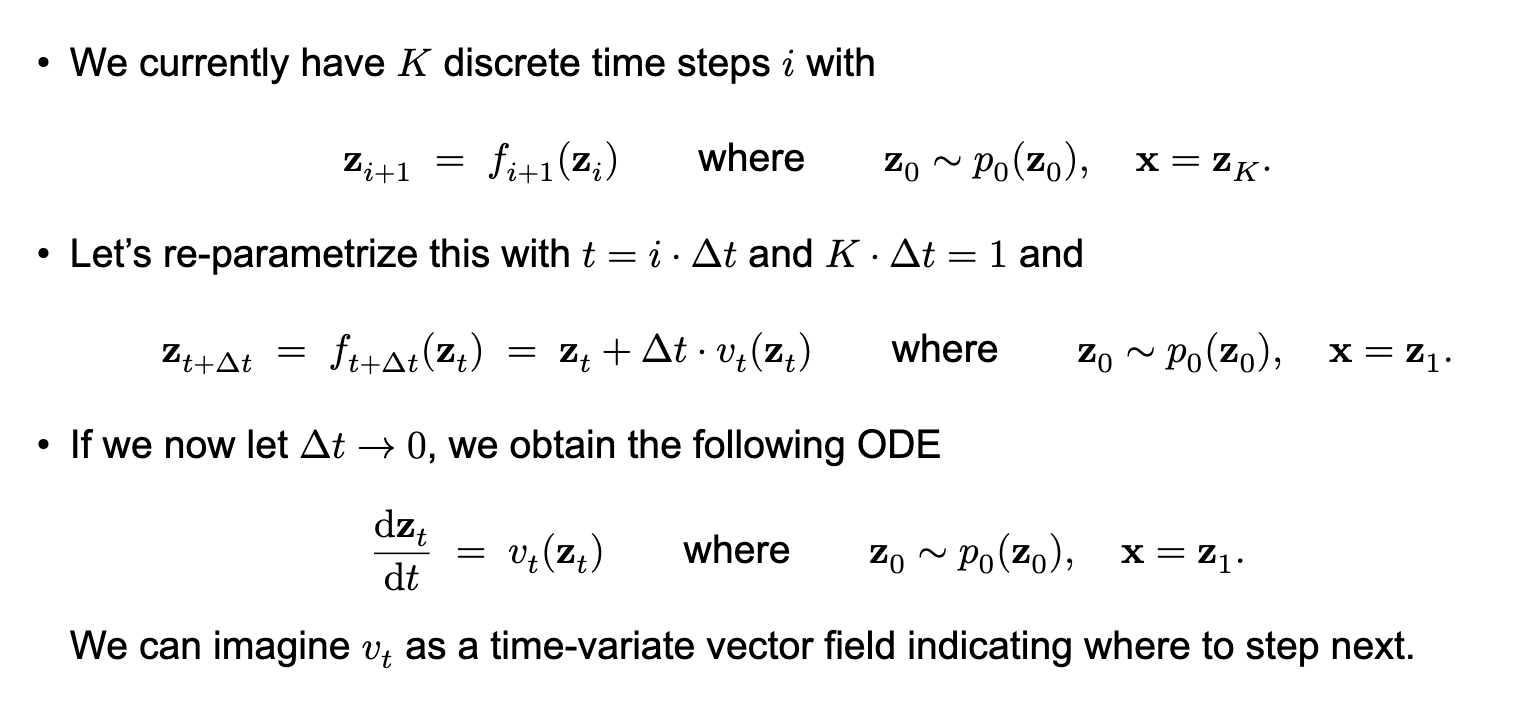 Problems: to train CNFs we need to deal with ODEs which is complex! can’t we approximate the true vector field and take a squared error?
 - We choose parametrized Gaussian path to approximate the true vector field
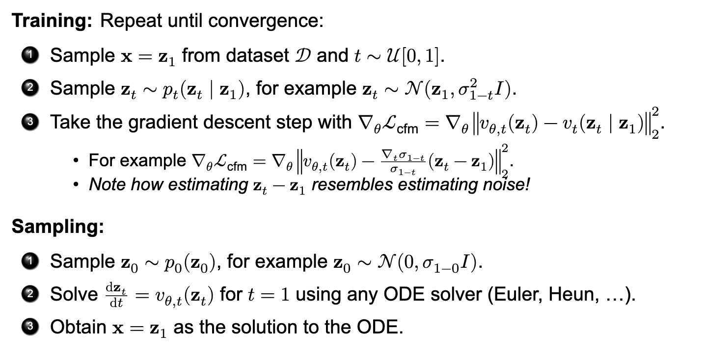
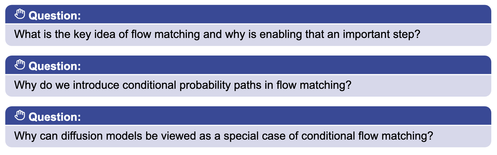
- Learn the vector field directly instead of using likelihood estimator or ODE solver, which turns generative modeling into a simple regression problem and generalizes diffusion models
- as the true vector field is unknown, we use conditional paths that provide vector fields that we can use as training targets
- diffusion models correspond to particular choices of probability paths. Variance exploding and variance preserving diffusion models are examples of such choices!
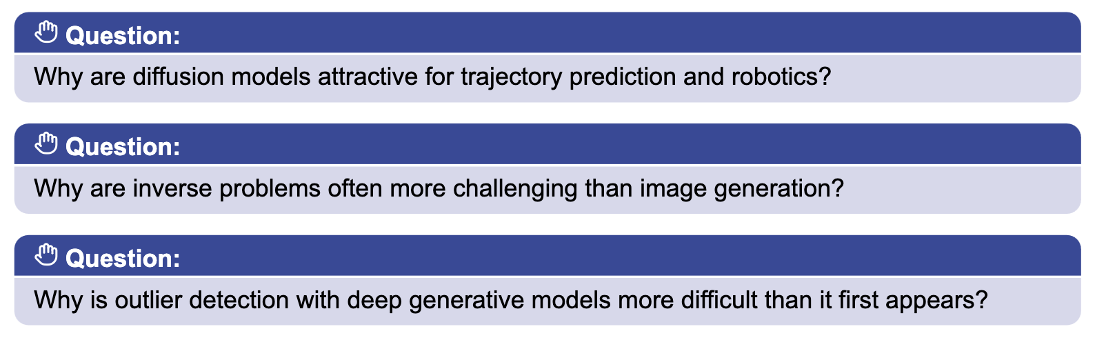
- because diffusion models can represent multiple plausible futures instead of producing only a single pred
- the goal is to not just generate a plausible result, but to also faithfully reconstruct the true underlying signal
- high likelihood does not necessarily mean that a sample belongs to the target dist!
Links:
202609022007