NERF
-
Novel view synthesis
-
problem - given a set of images with calibrated camera poses.
-
train a scene representation allowing us to easily predict a new image of the scene using an unseen target camera pose.
-
application - entertainment - AR/VR, real world perception, simulating novel scenarios - autonomous driving
-
how to obtain calibrated camera poses?
- use structure from motion methods ex-COLMAP
- a calibrated camera pose contains everything needed to project 3D points into the image which includes the camera’s position, orientation, and typically its intrinsic parameters such as focal length.
- it tells where the image was taken from, by allowing us to relate observations across different views and reason about the 3D structure of the scene hardly, as a single image only provides a part of the scene and limited geometric info!
-
-
Neural Radiance Fields (NeRFs)
-
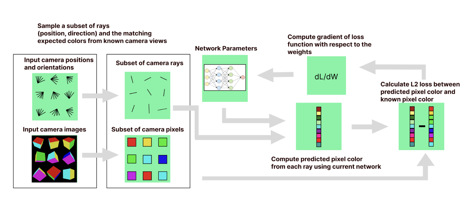
we cast rays into the scene from the camera ex - 1 ray per pixel using a pinhole camera model
-
and obtain color info in that direction.
-
For NeRFs the color is determined via simplified volumetric rendering techniques
-
Volumetric Rendering equations:
- absorption - radiance absorbed in a specific location (through particle)
- out-scattering - rad scattered in different direction
- emission - rad emitted at a specific location
- in-scattering - rad scattered in from other dir and sources
-
Radiance in NeRFs:
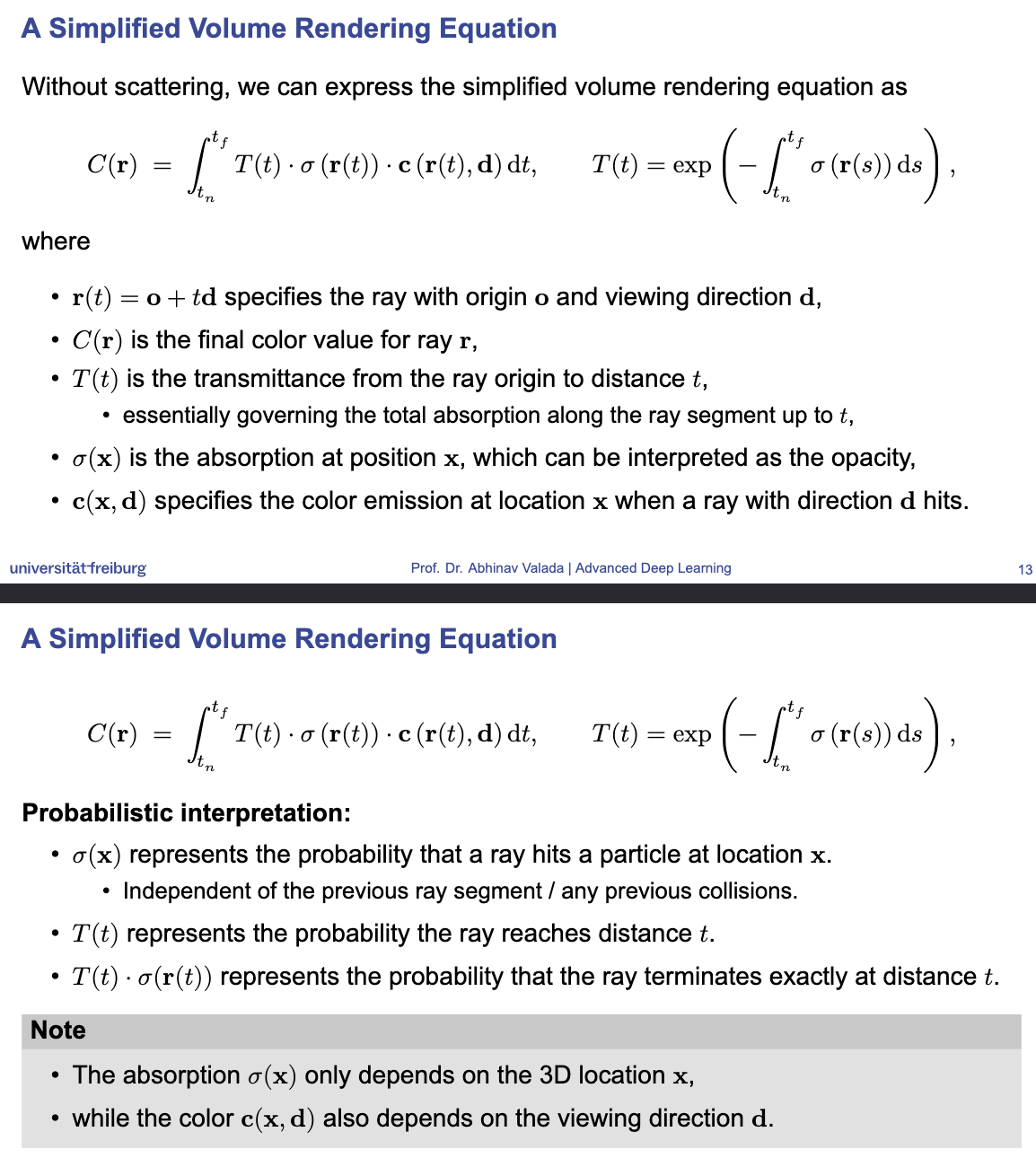
- we simplify and ignore out and in-scattering
- we do not deal with radiance directly and use just RGB color values
-
The idea is to learn c(x,d)- color and sigma(x) - absorption with a neural network
-
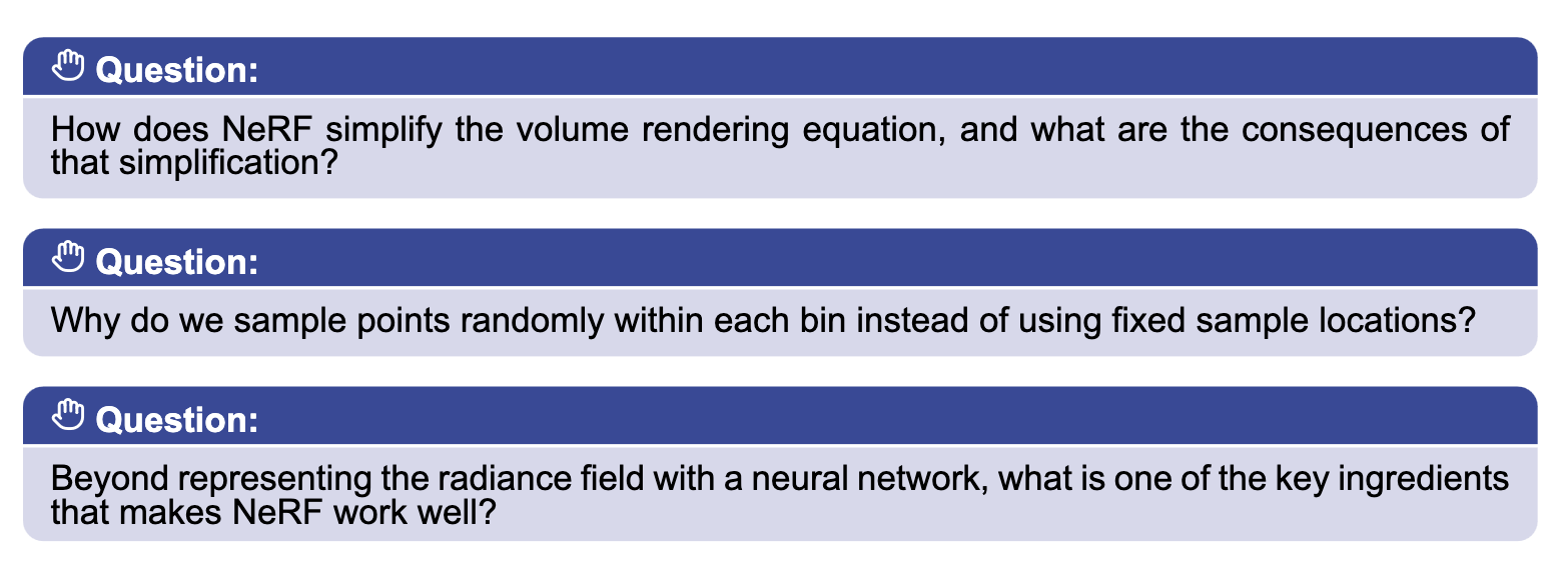
instead of calculating the integral we sample distances randomly from bin to not constraint the network to fixed discrete bin locations using traditional alpha-blending
-
Neural Radiance Field - Composition
- we sample N points along each ray
- input pos = (x,y,z) and direction d=(theta, phi) into radiance field model to obtain colors and densities
- compose the final ray colors via the discretized volumetric rendering equation
- train the network with an L2 loss against the ground truth colors.
-
problems:
- uniform sampling is inefficient
- detailed volume/border regions need more samples than empty space
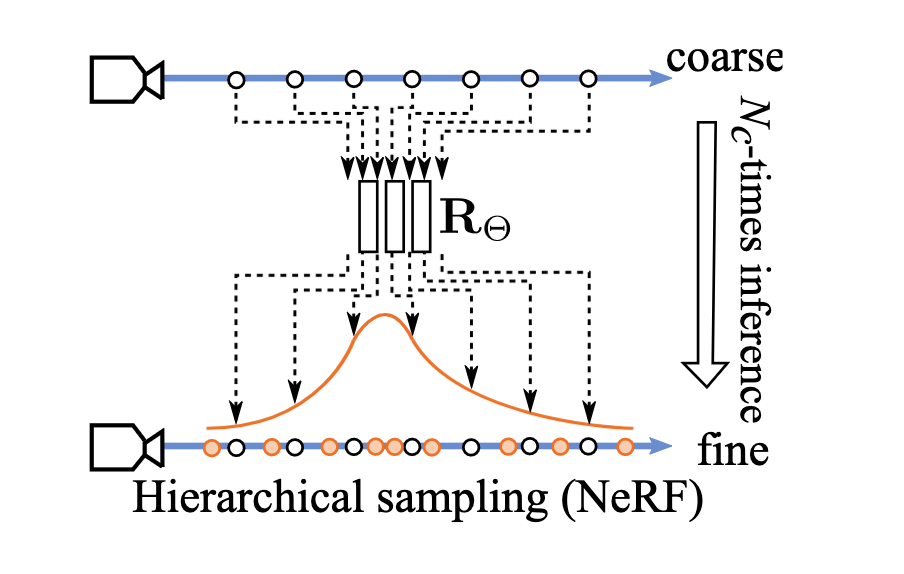
- therefore we train a coarse and a fine model
- sample the coarse model uniformly along the ray to obtain volumetric density
- then use this to create a coarse probability density function for the ray and finally use this probability density to sample with finer model!
- Hierarchical Volume sampling
-
NERF architecture
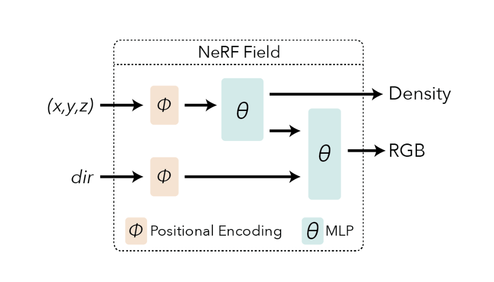 Density → depends on position
Color (RGB) → depends on pos + viewing dir
Density → depends on position
Color (RGB) → depends on pos + viewing dir- NeRFs depend on sinusoidal pos encoding for inputs without which we might get blurry results. Positional encoding allows NeRFs to capture high freq variations
- The color depends on viewing direction without which specular highlights disappear
→ how we train the network?
-
- it simplifies the volumetric rendering equation by removing the in and out scattering terms and only keeping the absorption and emission terms! reflection and scattering effects are therefore not modeled explicitly
- it helps the network learn continuous scene representation and prevents the network from memorizing values at specific locations and helps avoid discretization artifacts
- positional encoding which helps the network to represent high-frequency details that would otherwise appear blurry.
- 3D Gaussian Splatting
- NeRFs are slow to train (takes several days for a single scene)
- NeRFs are slow at rendering (upto 1 min per frame)
- geometry and scene are encoded implicitly
-
idea - represents the radiance field with anisotropic 3D gaussians
-
we parametrize each gaussian with:
- mean and covariance matrix
- opacity
- view dependent color
-
we can then computer color and density by blending together all Gaussians in our scene!
-
Rendering:
- instead of tracing a ray through scene we project or splat the 3D gaussians onto the 2D plane also called as rasterization!
- we can project the mean (of the gaussian) and the covariance (how spread the gaussian is) using transformation matrices and view projection
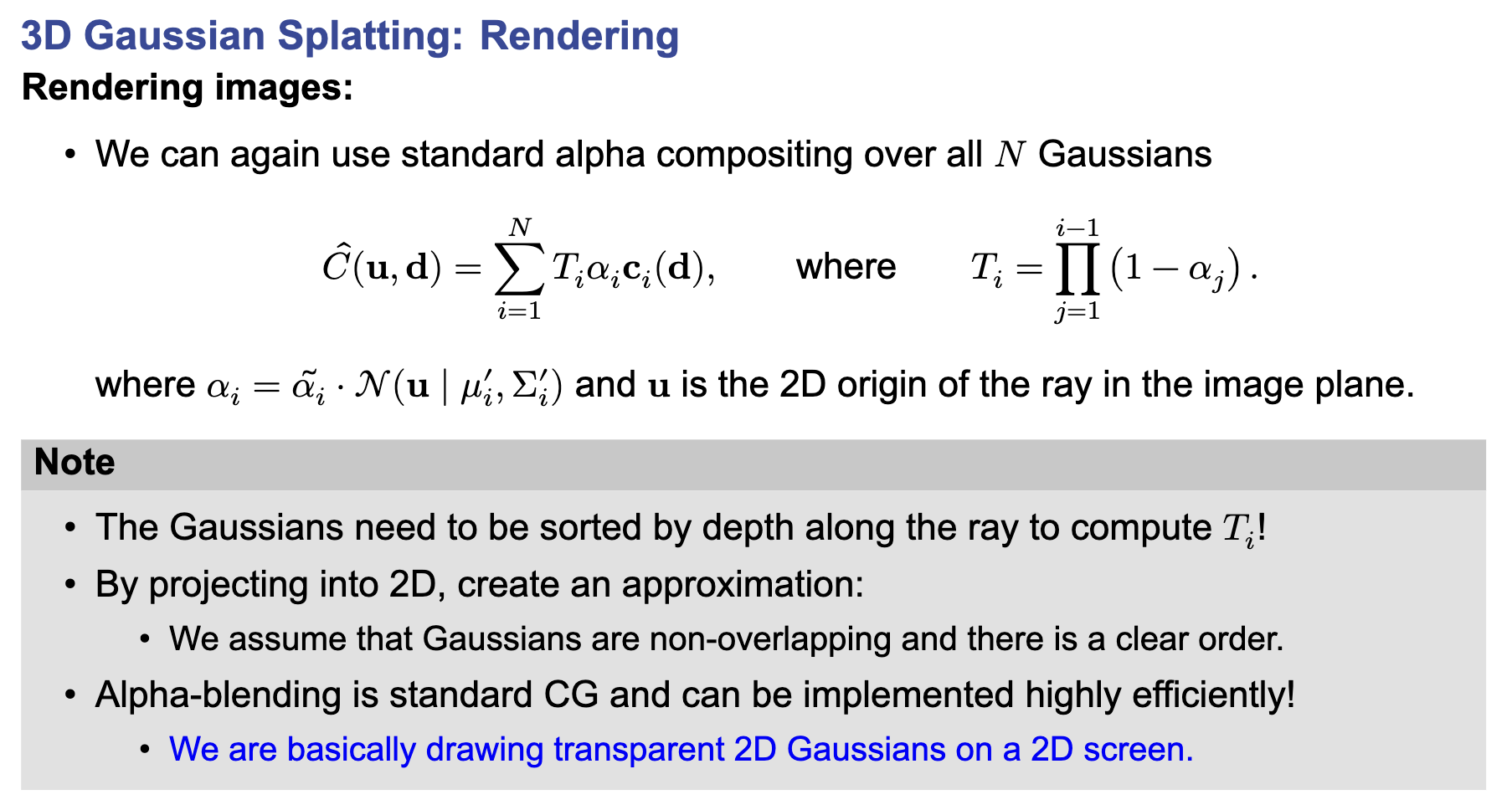
- then we only need to render 2d gaussians using standard alpha-composting (aka alpha blending)!
- the gaussians need to be sorted by depth along the ray to compute Ti (transmittance - which means the fraction of light that successfully passes through all layers in front of layer i)
- by projecting into 2d, we assume all gaussians are non-overlapping and there is a clear order.
- Alpha-blending is standard CG and can be implemented highly efficiently by drawing transparent 2D gaussians on 2d screen!
-
here Ti means how much light is reaching to the viewer ultimately after passing through all the gaussians in the ray! and C is the final color at the pixel which is the sum of each layer’s color ci, scaled by its opacity alpha and the light that actually reached it Ti
4-step method to render gaussian splatting:
- project the 3d gaussian into 2d (splatting)
- sorting by depth (i.e. sort the 2d gaussians by their depth along the viewing ray) which allows the transmittance Ti in the exact front-to-back order
- calc the pixel opacity which is calc as - max opacity at center (ã) x prob density of the gaussian
- alpha blending to get the final pixel color
parameters that need to be handled carefully:
- covariance needs to be pos semi-definite
- ã needs to be between 0 and 1
How to control the number of gaussians?
Adaptive Density Control:
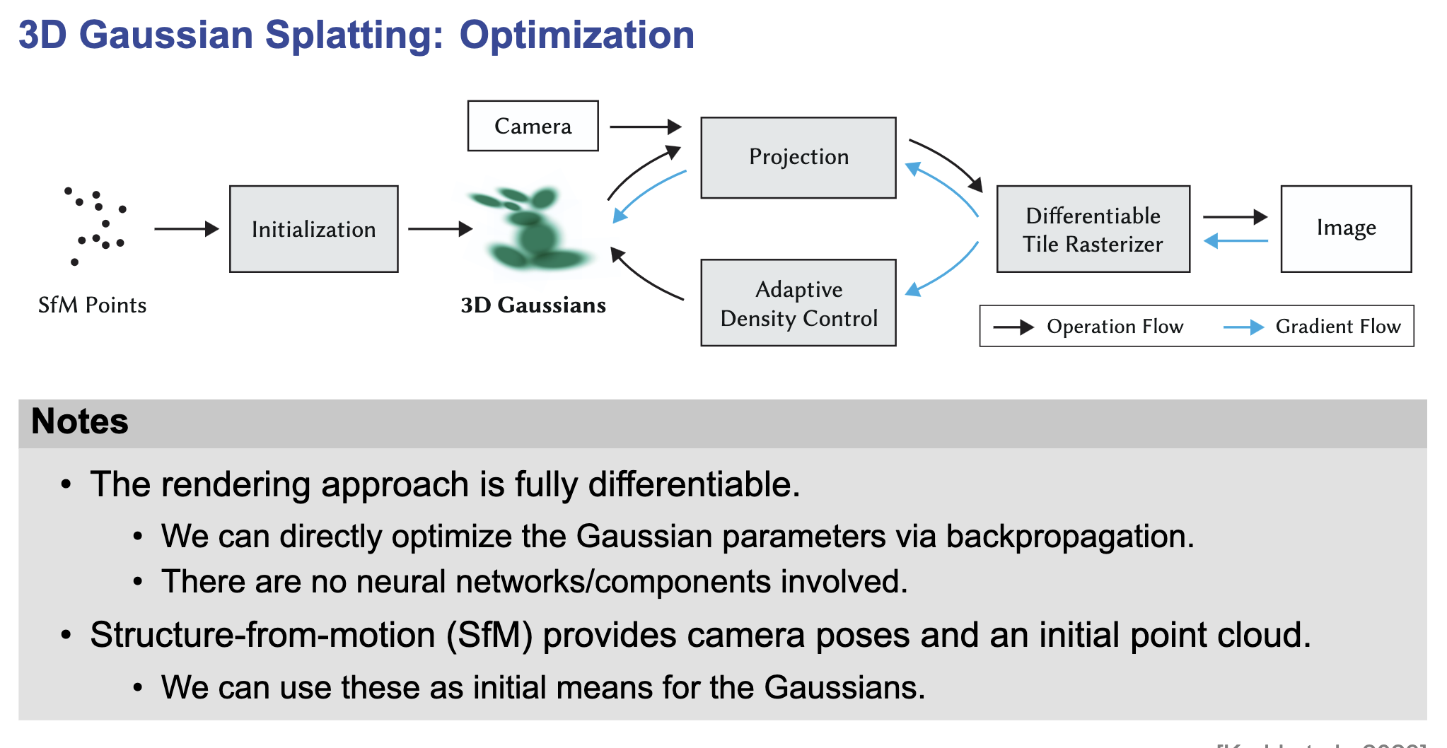
- for every K training steps, check if we should add or remove Gaussians
- if ã becomes too small (below a threshold) remove the gaussian
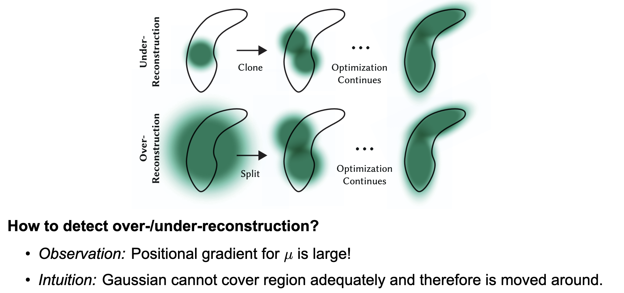
- add a gaussian if objects are over or under reconstructed
- under-reconstructed - small gaussian cannot cover the whole object (clone it and offset it by pos gradient)
- over-reconstructed - large gaussian covers more than the object (split it and re-position)
- NeRF uses ray tracing and uses a neural network to learn the scene implicitly while Gaussian splatting uses an explicit 3D point cloud of gaussians without using a neural network
- position, covariance, opacity, view-dependent color
- None, gaussian params are optimized directly through backpropagation without using any NN.
- World Models
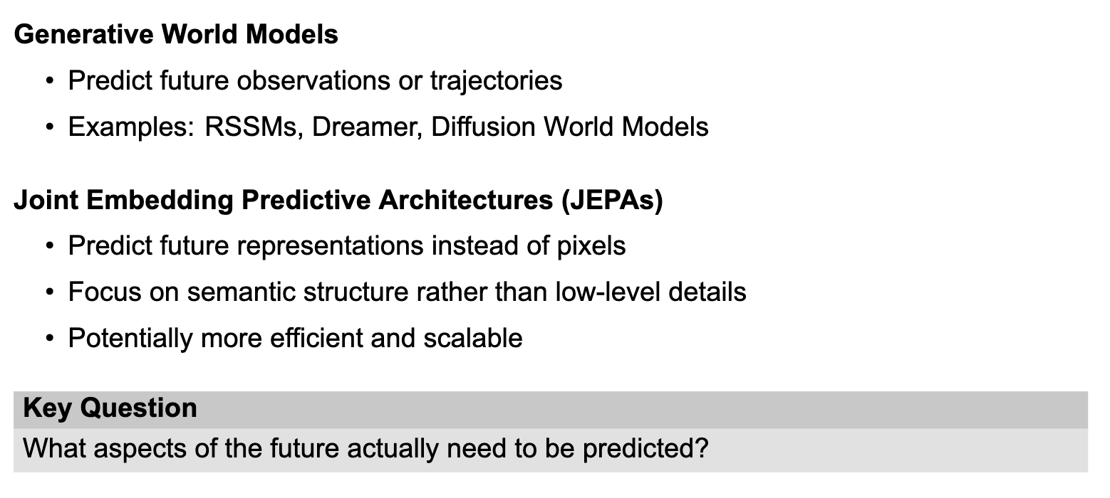
- a model that learns how the world works well enough to predict what might happen next
- feat of world models:
- the curr state of the world
- how the world changes over time (dynamics)
- how the actions affect future states
- uncertainty about the future!
- world models can imagine futures for planning, learning and safe-exploration
- Neural Scene representations describes what the world looks like in a fixed scene state whereas World models can think how the world might evolve, predict possible futures, and act as a learned simulator
- We can learn an env and generate imagined rollouts (dreams) and train an agent inside the dream!
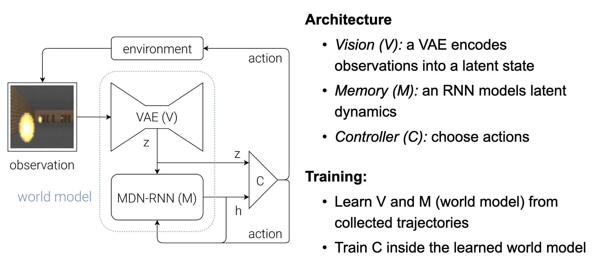
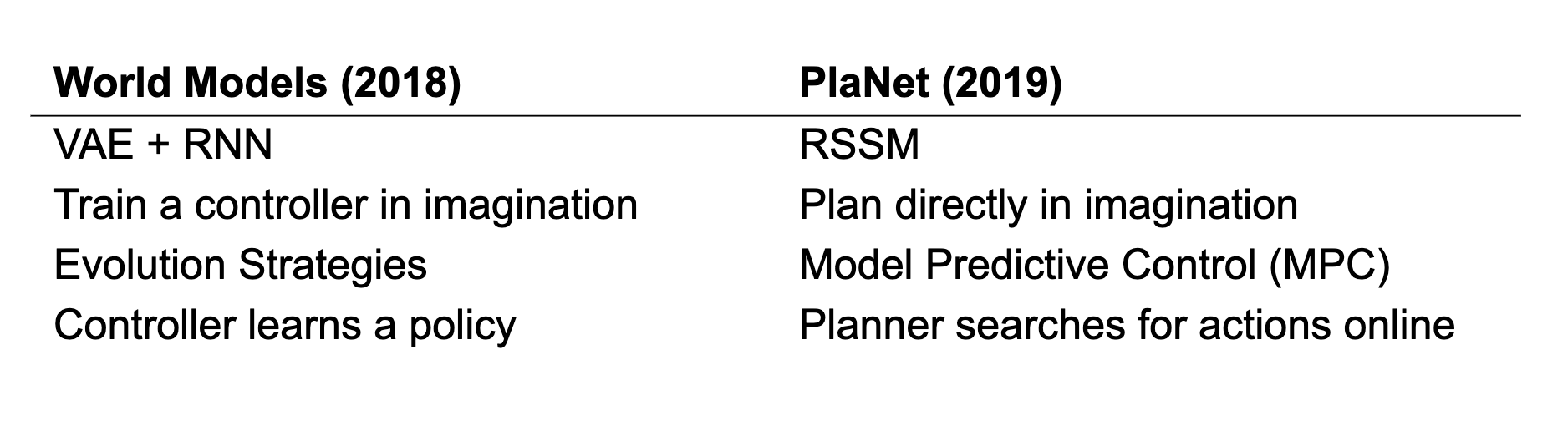
World models (2018)
-
Vision - learn a latent repr using VAE
-
Memory - predict future latent state using an RNN
-
Controller - train a controller inside imagined rollouts limitations:
-
the RNN hidden state must simultaneously represent
- mem of past
- uncertainty about present
- possible future outcomes
-
this makes modelling complex and uncertain environments difficult because deterministic vector has no built-in way to model probability distribution natively
-
RSSM - Recurrent State Space Models (separate memory and uncertainty)
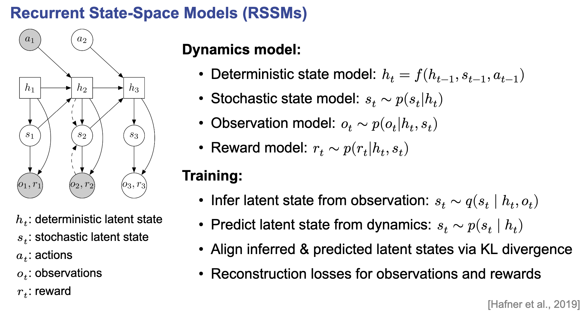
- introduced in PlaNet and utilized in Dreamer (v1 to v3) - RSSMs solve this bottleneck by explicitly separating deterministic memory from stochastic uncertainty
- RSSM maintains dual state representation at every timestep:
- Deterministic state - long term memory + context
- Stochastic state - current state + uncertainty + multiple plausible futures
Training of RSSM:
- KL Divergence Alignment - the predicted prior distribution p is forced to closely match the inferred posterior distribution q. This ensures that when the model is dreaming in the future without observations, its pure predictions remain physically realistic!
- Reconstruction loss - both the reconstructed observation and the pred reward must match the real data
-
PlaNet - Planning in Latent Space
- plan directly in the latent space not in the observation space
- learn a latent world model using RSSM
- predict future latent states and rewards
- evaluate candidate action sequences through imagined rollouts
- select actions with the highest predicted reward
- replan at every time step using the latest observation
-
Latent rollouts are significantly more efficient than predicting future observations
-
Dreamer
- PlaNet uses online planning via MPC - model predictive control
- online planning needs many imagined rollouts for every decision
- dreamer learns a policy and value function from imagined trajectories (training in dreams)
- actions are selected directly using the learned policy
-
Dreamer v2:
- discrete latent states
- improved training stability
- scales to Atari
- competitive with model-free RL
-
Dreamer v3
- robust training across domains
- single hyperparam config
- Atari, robotics, Minecraft
- Minecraft diamond benchmark
-
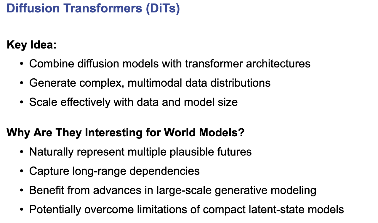
Limitations of RSSM:
- RSSM have been highly successful:
- efficient latent space prediction
- strong performance in planning and reinforcement learning
- PlaNet and Dreamer use RSSMs
- Challenges:
- long horizon prediction
- modeling highly multimodal futures
- scaling to increasingly complex environments
- exploiting advances in modern generative models
- RSSM have been highly successful:
- World models predict the future from the past
- Diffusion models are typically trained to generate an entire trajectory jointly
- Future and past are treated symmetrically:
- no notion of causality
How can diffusion models be adapted for causal prediction? because a physical world model must strictly predict the future conditioned on the past!
- Diffusion Forcing - trains the model by assigning different noise levels to different timesteps!
- past tokens are kept clean while future tokens receive more noise
- this assymetry forces the model to learn causal, step-by-step future predictions
Dreamer v4
- scale world models using transformer arch and diffusion based sequence modeling
- overview:
- transformer based world model
- causal sequence prediction via diffusion forcing
- shortcut forcing enables efficient inference
- improved long-horizon prediction and complex interactions
- enables training from large offline datasets
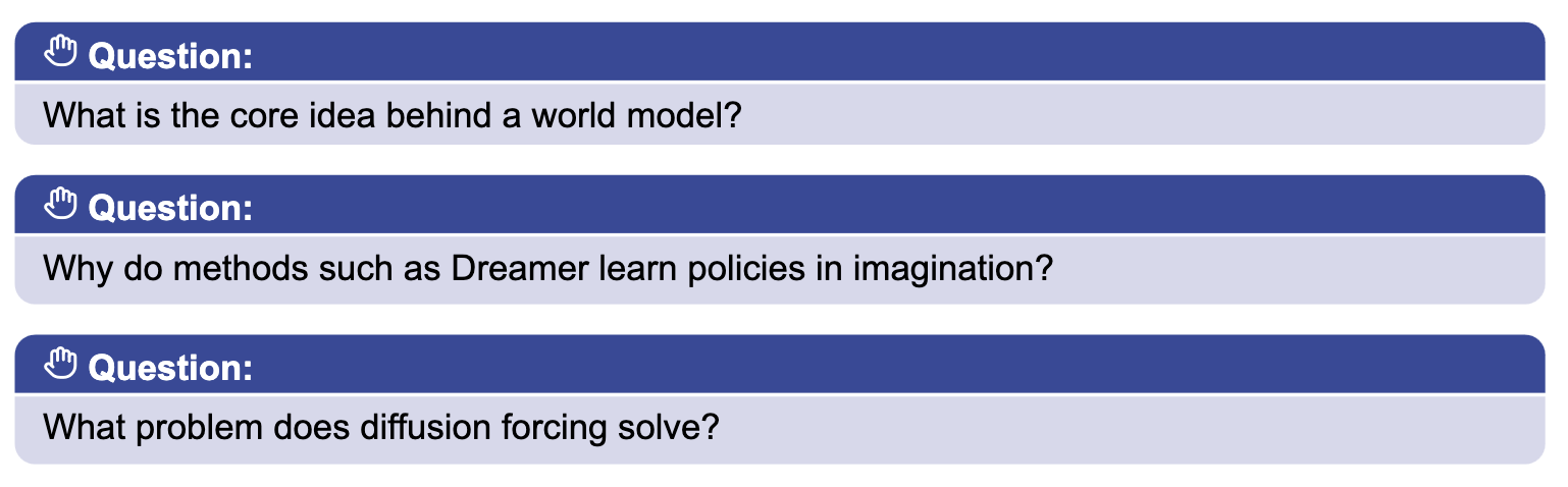
- learn predictive model of the env that can be used to imagine future states without interacting with the real world
- imagined trajectories are much cheaper and safer than real interactions, enabling more sample-efficient reinforcement learning
- diffusion forcing solves the problem that Diffusion transformer models jointly predict a trajectory without considering the past state or causality, diffusion forcing enables future prediction conditioned on a known past!
- Applications
Links:
202609041334